As if last week’s announcements of new Higgs results, B-dimuon decay, the rediscovered Y(4140), and all sorts of other goodies at HCP 2012 weren’t enough, there’s more big news from the world of experimental particle physics this week. A paper published just a few days ago in Physical Review Letters (here’s the PDF, and the arXiv page) describes the first observation ever of actual time reversal asymmetry: a difference between the behavior of a particular physical process and the time-reversed version of the same process.

Lest you get too excited, though: this has nothing to do with actual reversing of time, so it doesn’t mean time travel is possible or anything like that. And in fact, nobody in physics is the least bit surprised that it worked out the way it did. There is a theorem in physics called the CPT theorem (or sometimes PCT, or TCP, but not that TCP) which basically guaranteed that time reversal asymmetry had to show up somewhere. The theorem is suddenly getting a lot of attention in the news coverage of the discovery, but it’s technical enough that most people aren’t bothering to explain it. I’m going to fix that.

Discrete symmetries

The CPT theorem has to do with discrete symmetries. So first, let me explain what a discrete symmetry is, in the context of the laws of physics.

Imagine a rectangle.

This rectangle is symmetric in a few different ways. You can rotate it by 180 degrees, or you can flip it horizontally or vertically, and it still looks the same.

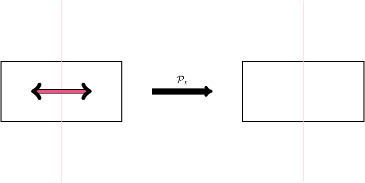
These are all examples of geometric discrete symmetries: transformations that you can make that don’t change the shape. They’re discrete because there are only a few specific transformations you can make that leave the shape unchanged — for example, if you’re rotating the rectangle, you can’t just rotate it by any old amount to get back to the same rectangle you started with. It has to be a multiple of 180 degrees. (Contrast this to, say, a circle, which you can rotate by any amount without changing it; that’s an example of a continuous symmetry.)

Of course, any geometric shape can also be specified as an equation. For the rectangle, you could write the following set of equations:

Perhaps not the most elegant set of equations, but it gets the job done. Anyway, the equations themselves aren’t that important. The point I want to make is that, just as shapes can be represented algebraically, so can transformations. Flipping the entire plane horizontally corresponds to reversing the sign of the \(x\) coordinate, and you can see that when you do that in the equations above, nothing changes. Similarly, flipping the plane vertically corresponds to reversing the sign of \(y\), and again, that doesn’t change anything in the equations. Rotating by 180 degrees is represented by a reversal of both signs; of course, again, the equations of the rectangle are unchanged.

Parity inversion

Let’s label these three transformations as \(\mathcal{P}_x\) for a horizontal flip, \(\mathcal{P}_y\) for a vertical flip, and \(\mathcal{R}_\pi\) for a 180 degree (\(\pi\) radian) rotation. \(\mathcal{P}\) stands for parity inversion, which is a transformation that changes the sign of one spatial coordinate. It’s the same P that appears in the name of the CPT theorem.

If you’re familiar with linear algebra, you probably know that each of these transformations can be represented as a matrix. For example, the horizontal flip takes \((x,y)\to(-x,y)\), and it’s not hard to figure out that the matrix \(\bigl(

If you’re not familiar with linear algebra, that’s okay. You can just think of \(\mathcal{P}_x\) as “horizontal flip” or \(x\to -x\) and ignore the matrix representation, and similarly for the other transformations.

Now, you may notice that, although I’ve identified two parity inversion symmetries of the rectangle (x and y), physicists talk about parity inversion symmetry (P symmetry) without specifying which direction it’s in. That’s because different parity inversions are really just rotated versions of each other. For example, flipping the plane horizontally is equivalent to flipping it vertically and then rotating it by 180 degrees.

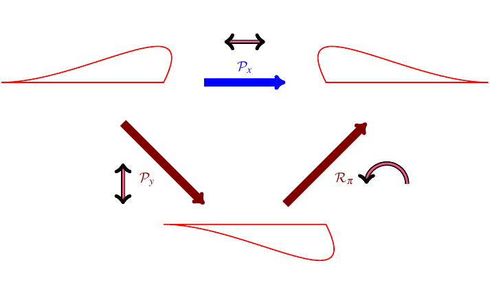
Mathematically, you could write this as

So out of these three discrete symmetries, only two of them are really independent. A version of this works for higher-dimensional spaces too, and also even if you don’t limit yourself to 180 degree rotations: in every case, all parity inversions in all possible directions are rotated versions of each other.

This particular tidbit is important because it allows us to only consider one parity inversion in the CPT theorem. Yes, I know I haven’t even explained what the theorem is yet, but so far we do know that it is a statement about transformations, and that one of them is parity inversion. So why can we get away with simply CPT rather than CPxPyPzT?

Well, the CPT theorem is a statement about Lorentz invariant quantum field theories (QFTs). Part of Lorentz invariance is rotational symmetry, which means that the laws of physics don’t depend on spatial orientation. Now, suppose a particular QFT also has parity inversion symmetry in the x direction, so that its laws don’t depend on the orientation of the x axis relative to the others. You can imagine rotating space by 180 degrees in the xy plane (which doesn’t change the laws), flipping it in the x direction (which doesn’t change the laws), and rotating it back (which doesn’t change the laws), and you wind up with an environment where everything is effectively mirrored in the y direction, but yet the physical laws are the same. That demonstrates that this theory also has parity inversion symmetry in the y direction. The same goes for any other direction: one parity symmetry plus rotational symmetry gives you all parity symmetries.

Time reversal

Quantum field theories are based on special relativity, and you may know that in relativity, time and space get treated on an equal basis (in some ways). If there’s a transformation (parity) that flips the orientation of one spatial direction, is there also one that flips the orientation of a temporal direction? Indeed there is. We call it time reversal, and the corresponding operator is \(\mathcal{T}\), which you can think of as “flip in time” or \(t\to -t\). Or if you prefer, you can construct a matrix representation of this operator the same way we did for parity (but I won’t here). This is, of course, the T in CPT.

While we’re on the subject of time reversal, I want to mention (again?) that when I talk about an operator that reverses time, I don’t mean that physicists actually have some way of making time run backwards. And similarly, with parity transformations, I don’t mean that we actually would flip the orientation of a spatial direction. These are all purely mathematical operators; all they let us do is play with the equations and see what would happen if, somehow, we could reverse time or space.

Charge conjugation

We have only one letter left: C, which stands for charge conjugation. This is the least intuitive of the three transformations, because it doesn’t change space or time; in fact, it doesn’t change anything easily visible. What it does is replace particles with antiparticles and vice-versa. (Almost. There is one caveat I’ll mention later.) Physically, this looks quite dissimilar from parity inversion and time reversal, but you can think of this as flipping some abstract mathematical “dimension,” so in a technical way, it’s not that dissimilar to the other transformations.

I’ll explain in some more detail what charge conjugation does, but first I have to explain fields.

Symmetries and fields

In the description of parity inversion above, I used a rectangle as an example. A rectangle is just a set of points, and transforming it is just a matter of rearranging the points. In field theories (quantum or otherwise), though, points are more than just points; they have values attached. The values can in general be anything: numbers, vectors, tensors, colors, etc. (although fields with non-mathematical values like colors aren’t much use in physics). So in a field theory, you can think of a spatial transformation as either rearranging the points, or as changing the value attached to each point. For example, the horizontal flip \(\mathcal{P}_x\) can be thought of as “change the value attached to the point at \((x,y)\) to the value that was previously attached to \((-x,y)\),” or in mathematical shorthand, \(\mathcal{P}_x[\phi](x,y) = \phi(-x,y)\). Here’s how that works on a color field.

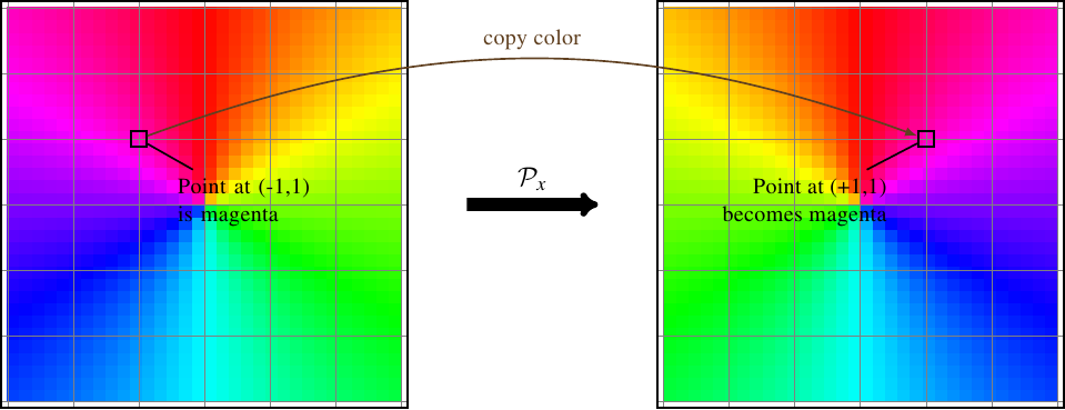
Sure, this description is a little harder to visualize, but thinking about transformations as changing values rather than locations lets you do more than just rearranging points. You can also do things like, say, double the value at every point in space, or subtract adjacent values.

Charge conjugation is one of these more general transformations. In a typical quantum field theory, each point is associated with one value for each kind of particle, which represents the amplitude for finding that kind of particle there. (Amplitude, \(\mathcal{M}\), is basically the square root of probability density \(P\), with some complex phase factor, so that \(\conj{\mathcal{M}}\mathcal{M} = P\).) The operation of charge conjugation swaps the values associated with each individual point for a particle and its antiparticle. For example, suppose the values associated with one particular point are

If you perform a charge conjugation, this swaps the values in each particle-antiparticle pair:

Since the photon is its own antiparticle, its value is unaffected.

Well… except for that one caveat I mentioned earlier. This is something that is mostly irrelevant for the level of detail I’m discussing this at, but it is important in the actual theory, so I mention it as a disclaimer to keep physicists from complaining at me. Particles in nature come in left-handed and right-handed varieties, and the opposite of a particle is its opposite-handed counterpart — for example, the antiparticle of a left-handed electron is a right-handed positron. And charge conjugation doesn’t change the “handedness” of a particle. Parity inversion does, though, so you can combine \(\mathcal{C}\) and \(\mathcal{P}\) to convert a particle into its actual antiparticle.

Accordingly, if a theory has the same laws for particles and their antiparticles, we call that CP symmetry.

The CPT Theorem

Now that I’ve explained all the transformations involved, I can get on to the CPT theorem itself. The theorem isn’t actually all that complicated, once you know what the transformations are. All it says is that if you take any Lorentz invariant quantum field theory (basically any QFT that obeys relativity), and mathematically flip particles to antiparticles (\(\mathcal{C}\)), flip one spatial dimension (\(\mathcal{P}\)), and flip the time dimension (\(\mathcal{T}\)), you’ll arrive back at a theory with exactly the same laws of physics as the one you started with.

Proving the CPT theorem is not especially complicated either, but it is tedious: you just go through each of the possible terms that can occur in a generic Lorentz invariant quantum field theory and show that if you apply the transformation \(\mathcal{CPT}\) to the fields, all the changes cancel out. The nature of the proof isn’t really important, though. What is important is that it works for any Lorentz invariant QFT, regardless of the details. The only way this theorem could be false is if Lorentz invariance (basically, relativity) doesn’t work, or the entire framework of quantum field theory doesn’t work, and there are boatloads of evidence to suggest that neither of those two things is the case.

History of discrete symmetry violation

So if we know that this composite transformation \(\mathcal{CPT}\) can (mathematically) be made without changing the basic laws of physics, what does that mean? Well, back in the old days (the 50’s), it didn’t seem to be a big deal, because physicists thought that none of the three transformations individually could change the laws of physics. In other words, they thought the laws of physics couldn’t depend on spatial orientation, or on the direction of time, or on whether you’re dealing with particles and antiparticles. And who can blame them, because particles did seem to act just like their antiparticles, and left seemed to act like right, and all the other laws of physics were symmetric in time so why wouldn’t QFTs be?

But nature is tricky! In 1957, a group led by Chien-Shiung Wu found that some particles don’t behave the same as their mirror images. They measured the decays of radioactive cobalt atoms which were all spinning in the same direction, and found that the radiation all came out in one direction, never the other. If you could apply a parity inversion to nature, then you would come up with a world where the radiation all came out in the other direction. Not the same! So clearly, a parity inversion does change the actual laws of physics. We say that parity inversion symmetry is violated in the standard model (the particular QFT that best matches reality), or for short that the standard model exhibits parity violation.

It wasn’t long after that until physicists discovered CP violation, which is that the laws of physics do not treat particles and antiparticles the same either. In 1964, James Cronin and Val Fitch measured a difference in the decays of K mesons and their antiparticles. Since decays are a very direct probe of the fundamental laws, this was a clear case of those laws treating particles and antiparticles differently.

So as of the 1960s we knew that, if you mathematically switch particles to antiparticles, you change the laws of physics. But we know that if you mathematically switch particles to antiparticles and reverse time, you do get back to the same laws you started with. This means that the time reversal has to undo the changes to the physical laws caused by the particle-antiparticle switch, and that’s why physics cannot be time reversal invariant. As you might imagine, physicists have been very interested in finding direct evidence of this time reversal asymmetry.

Of course, it’s easier said than done. (And that’s saying something, because it hasn’t exactly been easy to say!) Because we can’t actually reverse time, the only way to find evidence of time reversal asymmetry is to look among the physical processes that to break these symmetries (like the B meson decays) and find one for which both it and its time-reversed counterpart can be made to occur. Unfortunately, those two criteria tend not to occur together. The only interaction that breaks symmetries is the weak interaction, and weak interactions are mostly just decays. When a particle decays, it produces a bunch of products that fly away in all directions, some of which are unstable or even undetectable! Controlling all those particles well enough to shoot them back together in a backwards decay just isn’t possible. So for a long time physicists weren’t sure they would ever be able to test this symmetry.

B meson oscillations

This is where the recently published experiment by the BaBar collaboration comes in. It’s the first unambiguous detection of a phenomenon that can only be explained by time reversal symmetry. The method they used is pretty clever, but it takes some careful thought to understand it. I’ll attempt to explain it, but if this isn’t clear, just keep in mind that it took me about three passes through the relevant papers to start to understand what was going on.

In a B meson factory like the one at BaBar, neutral B mesons and their antiparticles are produced in entangled pairs. Each B meson can decay in one of two ways (for our purposes): either “hadronically,” into two lighter mesons (\(J/\psi\) and a kaon), or “leptonically,” into a lepton and other stuff which we don’t care about. Since the particles are entangled, if they were normal particles, both of them would always decay the same way, either both hadronically or both leptonically, but never one and one. So, for example, if you see the first B meson decay leptonically, then normally that tells you the other one has been forced into a state such that it will also decay leptonically.

However, B mesons are not normal particles. They can oscillate, which means that even if a B meson is forced into a state which means it will decay leptonically, it will naturally change its state over time, and after a while it has a decent chance of decaying hadronically again. This oscillation is the time-reversal-asymmetric process that the BaBar paper measured. They picked out the times when the first B meson in a pair decayed leptonically, thus forcing its partner into a leptonic decay state, but the partner oscillated back to decaying hadronically, and also the times when the first B meson in a pair decayed hadronically and the partner oscillated back to decaying leptonically, and they compared how many times each one happened.

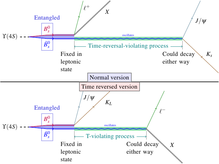
If the standard model were unaffected by time reversal, you’d expect these two measured counts to be the same. However, BaBar found that the leptonic to hadronic oscillation occurs significantly more often than the hadronic to leptonic oscillation in the time before the B meson decays. That confirms the time reversal symmetry violation.

These figures from the paper show asymmetry coefficients calculated from the measurements of how often each kind of transition occurred. In each case the red line is the prediction if time reversal symmetry is violated, and the blue line is the prediction if it’s not. It’s pretty clear that the red line is the better fit. In fact, if you run through the statistical analysis, the model with time reversal symmetry (blue line) is disfavored at a significance of \(14\sigma\)! So there’s effectively no chance of this being a statistical fluke: the probability that the experiment would produce this data without time reversal symmetry violation is a paltry \(\num{1.56e-44}\). You could run this experiment millions of times a second for the entire history of the universe and never expect to see something that unlikely happen, not even once.

Arrow of time

One last thing I want to mention: all this has nothing to do with the arrow of time. Just so that’s clear. In physics, “arrow of time” refers to the issue of why time flows forwards rather than backwards, and this measurement hasn’t shown that. All it has done is to show that the forward and backward directions in time are different, because the fundamental laws of physics look slightly different depending on which way in time you’re going. But just because the two directions in time are different, it doesn’t automatically single out one of them as the forward one.