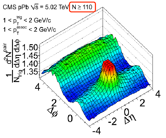
Over the past few days, the news about the LHC possibly discovering (or even confirming, in some sources!) a new kind of matter has popped up on quite a few websites — blogs, science news sites, Twitter, Google+, Reddit, elsewhere on Reddit, you name it. Of course, I was writing about this before it was cool :-) I reported the discovery of the ridge presented by CMS at the High pT LHC Physics Workshop. Back then it wasn’t clear that anyone really knew what was going on, but of course that important fact got lost in the hype.

As I posted in a more recent update, there is a lot of speculation that this ridge might have something to do with something called the color glass condensate (CGC). This is what so many sites are calling the new state of matter that the LHC has supposedly discovered. Well, I actually know something about this! Sort of. The CGC is an incredibly complex mathematical model, but it is somewhat closely related to what I work on, so I figured I could try to explain what’s going on in some more detail.

Parton distributions

All this starts with the question: what’s inside a proton?

“Three quarks!” you might say, and in a very simple sense, you’d be on the right track. But it turns out that a proton is a lot more complicated than three little particles flying around each other. See, a proton is so small that to get any real understanding of what it is, we have to look to quantum field theory.

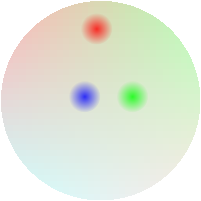
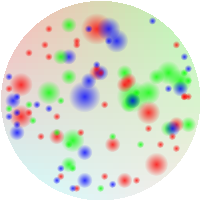
QFT says that the proton is really a coherent excitation in various quantum fields. But what is that? It probably doesn’t mean anything to you if you don’t know quantum field theory, and even if you do, an excitation in a field isn’t exactly the easiest thing to visualize. So instead, we tend to think of these excitations as particles, or groups of particles. This is an easier-to-digest, while still mathematically useful, view of the proton: it contains a complicated “sea” of a huge number of little particles, called partons. Not just the three quarks we’re used to thinking of, but also photons, quark-antiquark pairs of all types, and especially gluons, the things that are primarily responsible for binding the quarks together, kind of like how dough binds the chocolate chips in a cookie together.

These are quantum particles, so they pop in and out of existence randomly. So we can’t describe the contents of a proton by making an exact map of where the individual quarks and gluons are, the way we do with normal objects. And unlike an atom, which has everything except the electrons concentrated in the center, in a proton any constituent particle can show up anywhere. So the only way we can describe the content of a proton is statistically, with the probability that a given type of particle shows up with a given set of kinematic properties.

Over the past 30 years or so, when they haven’t been working on finding the Higgs boson or supersymmetry or other things you may have heard of, physicists have measured a set of functions, called parton distributions, that describe these probabilities. There’s one for each kind of quark, and one for gluons. Instead of giving the probability that a parton appears in a particular position, though, the parton distributions give the probability of finding one with a specific momentum (and energy), because it’s easier to calculate things that way.

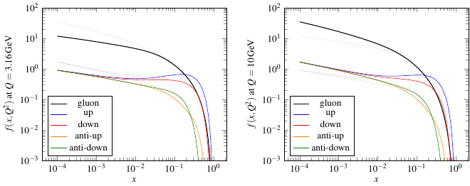
This plot shows a selection of parton distributions at various values of the kinematic variables \(x\) and \(Q^2\). Roughly, you can kind of think of \(x\) as being related to the energy of the probe that hits the proton — the smaller \(x\) is, the larger the energy — and \(Q^2\) is related to the amount of transverse momentum the probe transfers to the quark or gluon it hits. It’s like the strength of the sideways “kick” that knocks the parton out of the proton. (Kind of. It’s really more complicated than the kick — if I wanted to be technically correct, I’d say \(\vec{q}\) is the actual momentum transfer and \(Q^2 = -q^2\) — but I’m not thinking of a better nontechnical way to describe what \(Q^2\) is.)

Saturation and the CGC

In the plots above, you can see that the parton distribution for gluons shoots way up at small values of \(x\), which correspond to very high-energy collisions. That means basically that as you go to higher and higher energy collisions, the probe which hits the proton has the potential to interact with more and more gluons. It’s as if the proton is made up of varying numbers of particles depending on how hard it gets hit! Yes, it’s very strange to think about the composition of a particle changing depending on what you hit it with, but that’s just because we’re trying to force a particle-like description on to something that is actually a quantum field. It’s bound to not make sense in some ways.

Just as higher energy means more and more gluons, having a higher transverse “kick” means that the probe can interact with smaller and smaller gluons. Again, it’s as if the proton consists of smaller and smaller particles the more transverse momentum you hit it with. When you put those two trends together, you can make a picture of how the particle composition of the proton appears to change depending on the properties of the probe:

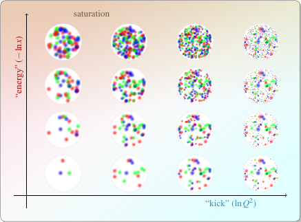
Check out the top of that picture, especially towards the left. You can see that the partons are getting pretty densely packed. And when they get densely packed, they’re going to interact with not only the probe, but with each other as well. That “self-interaction” among gluons modifies the way they behave in collisions in some interesting ways. We call this phenomenon of densely packed gluons saturation.

You can see this in the equations, too. Without saturation, so for example in the bottom part of the last picture, one of the equations that describes the behavior of gluons is the BFKL equation,

Here \(N\) is a function related to the gluon distribution I showed in the plot earlier, and \(\mathcal{K}\otimes N\) is an integral of some stuff times \(N\). When you include the effects of saturation, you have to add something to the equation:

This is called the BK equation. The details of the equation don’t matter so much for this post, but the point I want to make is that gluon self-interactions can be represented by a fairly simple term in the equation. (Don’t be fooled, though, actually solving this thing is a nasty affair despite its deceptively simple appearance.)

Just the fact the gluons interact with each other isn’t the whole story, though. There are also a lot of gluons, which means a lot of interactions, and that modifies their behavior even more in ways that aren’t apparent from just considering how individual gluons interact with each other. It’s kind of like how you can build a sand castle solid enough to stub your toe on out of millions of grains of sand, even though two of them won’t stick to each other — only of course, with gluons it’s much more complicated. It turns out that properly taking this kind of effect into account in the equations is not as simple as just adding a term. It needs a whole new equation — multiple equations, even, which involve whole new variables that don’t even appear in the BFKL or BK equations. (I don’t think there’s much point writing it down here, but look up the Balitsky-JIMWLK equations if you’re interested.)

The net effect of all this is that, when \(x\) is very small (which, remember, means high energy), the gluons have complicated interactions which tend to correlate their behavior, somewhat like how all the fish in a school move together. Collisions with different (large) energies look more similar than you’d expect by just extrapolating the behavior from low-energy collisions. This slowed-down evolution with energy, as we say, is similar to how glass changes its shape only abysmally slowly. In this sense, we call this high-energy behavior of gluons, and the mathematical model that explains it, the color glass condensate.

Evidence from CMS

I’ve already shown the evidence from CMS that could be interpreted as the first sign of the color glass condensate.

But of course, as I’ve been saying, it’s not definite yet. Even the original paper highlights two theoretical explanations. First, there is hydrodynamic flow, which is the same sort of thing that occurs in lead-lead collisions, only it wouldn’t be as strong in this case because not that many particles are involved in a pA collision. Here’s what the paper says about that (feel free to skim over it):

Long-range correlations in pPb collisions have been quantitatively predicted in models assuming a collective hydrodynamic expansion. The correlation resulting from the predicted elliptic and triangular flow components for pPb collisions at \(\sqrt{s_{NN}} = \SI{4.4}{TeV}\) are compared to the observed correlation in Fig. 2 for the \(1 < p_\text{T} < \SI{2}{GeV}/c\) selection (solid line, second column). The magnitudes for elliptic and triangular flow of \(v_2 = 0.066\) and \(v_3 = 0.037\) correspond to those given in Ref. [25] for the highest multiplicity selection and the average value of \(p_\text{T} \approx \SI{1.4}{GeV}/c\) found in the data. The same \(v_2\) and \(v_3\) coefficients were used for all multiplicity classes, showing the multiplicity dependence of the correlated yield assuming a constant flow effect. While this provides and indicative and useful illustration of the magnitude of the observed near-side enhancement, a detailed quantitative comparison of the model and data will need to include the additional non-hydrodynamical correlations from back-to-back jets, as well as the effects of momentum conservation, which suppress the correlation near \(\Delta\phi\approx 0\) relative to \(\Delta\phi\approx\pi\).

The figure they reference is this one:

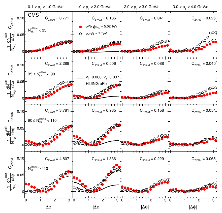
This shows the data collected as red dots, and the model they’re talking about is in the second column as a solid line. While it doesn’t seem to agree that well, it does get the rise on the left side of the graph near \(\Delta\phi\approx 0\), which is really the important part — on the other side of the graph, near \(\Delta\phi\approx\pi\), there are other things that could be causing the data to be higher than the model. (Those are the back-to-back jets mentioned in the description.) So this hydrodynamic flow hypothesis is something worthy of further consideration.

Meanwhile, when it comes to the CGC, the paper includes this:

The ridge-like structure in pPb collisions was also predicted to arise from initial state gluon correlations in the color-glass condensate framework. This model qualitatively predicts the increase in the correlation strength for higher multiplicity pPb collisions, although it remains to be seen if the large associated yield seen in the highest multiplicity selection can be quantitatively reproduced in the calculation.

(emphasis added) They’re saying that, like the hydrodynamic flow model, the CGC model does predict the fact that the ridge should form, and that it should get stronger at collisions involving more particles, which is indeed the trend they saw — but they don’t yet have enough data to check the prediction more precisely than that. So it’s still an open question whether the CGC is real or not.