Time for a blog post that has been far too long coming! Remember the Quest for B Meson Decay? I wrote about this several months ago: the LHCb experiment had seen one of the rarest interactions in particle physics, the decay of the \(\mathrm{B}^0_s\) meson into a muon and antimuon, for the first time after 25 years of searching.

Lots of physicists were interested in this particular decay because it’s unusually good at distinguishing between different theories. The standard model (which incorporates only known particles) predicts that a muon and antimuon should be produced in about 3.56 out of every billion \(\mathrm{B}^0_s\) decays — a number known as the branching ratio. But many other theories that involve additional, currently unknown particles, predict drastically different values. A precise measurement of the branching ratio thus has the ability to either rule out lots of theoretical predictions, or provide the first confirmation on Earth of the existence of unknown particles!

Naturally, most physicists were hoping for the latter possibility — having an unknown particle to look for makes things exciting. But so far, the outlook doesn’t look good. Last November, LHCb announced their measurement of the branching ratio as

In the months since then, the LHCb people have done a more thorough analysis that incorporates more data. They presented it a couple of weeks ago at the European Physical Society Conference on High-Energy Physics in Sweden, EPS-HEP 2013, along with a similar result from the CMS experiment. Here’s the exciting thing: the two groups were able to partially combine their data into one overall result, and when they do so they pass the arbitrary \(5\sigma\) threshold that counts as a discovery!

Yes, I am about to explain what that means. :-)

Without Further Ado

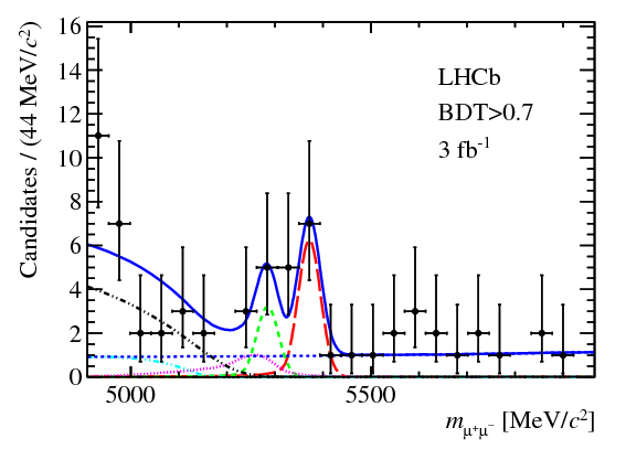
In this plot from LHCb,

and this one from CMS,

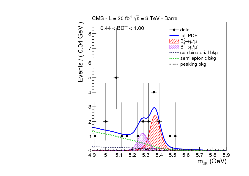
you can see the number of events detected in each energy range, the black dots, along with the theoretical prediction for what should be detected assuming the standard model’s prediction of the decay rate is correct, represented by the blue line. The data and the prediction are clearly consistent with each other, but that by itself doesn’t mean we can be sure the decay is actually happening. Maybe the prediction that would be made without \(\mathrm{B}^0_s\to\ulp\ualp\) decay would also be consistent with the data, in which case these results wouldn’t tell you anything useful.

A more useful plot is this one from the CMS experiment, which shows the likelihood ratio statistic a.k.a. log-likelihood (on the vertical axis) as a function of the branching ratio (or branching fraction \(BF\)):

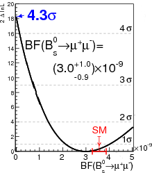
Basically, the plot tells you which values of the branching ratio are more or less likely to be the true branching ratio, using the measured value as a reference point. For example, CMS measured the branching ratio to be \(\num{3e-9}\), so in the absence of other information, that’s the most likely true value of the branching ratio. The most likely value is no less likely than itself (just meditate on that for a moment), so the curve touches zero — the bottom of the graph — at \(\num{3e-9}\).

On the other hand, consider \(\num{2.1e-9}\). That’s not the number CMS measured, so it’s less likely that the true branching ratio is \(\num{2.1e-9}\) than \(\num{3e-9}\). How much less likely? Well, if you look at the plot, the value at \(\num{2.1e-9}\) is pretty much on the \(1\sigma\) line. But you have to be careful how you interpret that. It does not tell you the probability that the true value is less than \(\num{2.1e-9}\), but it does tell you that, if the true value is \(\num{2.1e-9}\), the probability of having measured the result CMS did (or something higher and further away from the true value) is the “one-sided” probability which corresponds to \(1\sigma\): 16%. (That number comes from the normal distribution, by the way: 68% of the probability is within one standard deviation of the mean, leaving 16% for each side.) Yes, this is kind of a confusing concept. But the important point is simple: the higher the curve, the less likely that value is to be the true value of the branching ratio.

The most interesting thing to take away from this graph is the value for a branching ratio of zero, where the curve intersects the vertical axis. That tells you how likely it is that the branching ratio is zero, given the experimental data. (Technically zero or less, except that we know it can’t be less than zero because a negative number of decays doesn’t make any sense!) It’s labeled on the plot as \(4.3\sigma\). That corresponds to a one-sided probability of \(\num{8.54e-6}\), or less than a thousandth of a percent! In other words, if \(\mathrm{B}^0_s\to\ulp\ualp\) doesn’t happen at all, the chances that CMS would have seen as many \(\ulp\ualp\) pairs as they did is 0.001%. That’s a pretty small probability, so it seems quite likely that \(\mathrm{B}^0_s\to\ulp\ualp\) is real.

Let’s be careful, though! Because if you do run a hundred thousand particle physics experiments, you can expect one of them to produce an outcome with a probability of 0.001%. How do we know this isn’t the one? Well, we don’t. But here’s what we can do: estimate the number of particle physics experiments and sub-experiments that get done over a period of, say, several years, and choose a probability that’s low enough so that you don’t expect to get a fluke result in all those experiments. For example, let’s say there are 10,000 experiments done each year. If you decide to call it a “discovery” when you see something that happens with a probability of 0.001%, you’ll “discover” something that doesn’t really exist every ten years or so. But if you hold off on calling it a “discovery” until you see something that has a probability of 0.00003% — that’s one in 350 million — you’ll only make a fake discovery on average once every few centuries. Or in other words, once in the entire history of physics, since Newton! Physicists have chosen this threshold of a 1-in-350-million probability to constitute a “discovery” for exactly that reason, and also because it corresponds to a nice round number of sigmas, namely five.

So in order to say the decay \(\mathrm{B}^0_s\to\ulp\ualp\) has officially been discovered, we would need that curve on the plot to shoot up to \(5\sigma\) by the time it hits the vertical axis. CMS isn’t there yet.

The Combination

LHCb also has their own, separate result showing evidence for the decay. It’s natural to wonder, could we combine them? After all, if it’s unlikely that one experiment sees a decay that doesn’t exist, it must be way less likely that two separate experiments indepdently see it!

That’s true to some extent, but it’s not an easy thing to properly combine results from different experiments. You can’t just multiply a couple of probability distributions, because the experiments will often be made of different components, work in different ways, and have different algorithms for filtering and processing their data, and all of that has to be taken into account to produce a combined result. But in this case, the LHCb and CMS collaborations have decided their detectors are similar enough that they can do an approximate combination, which they shared during the EPS-HEP conference.

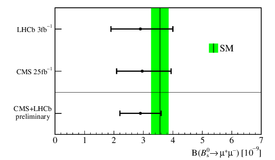
This plot shows the individual measurements and uncertainties from LHCb,

from CMS,

as well as the combined value,

and the standard model prediction in the green band,

The uncertainties are \(1\sigma\), which means the error bars indicate how far it is from the measured value to the point at which the log-likelihood curve passes the \(1\sigma\) mark. You can see that they match up in this composite of the two plots:

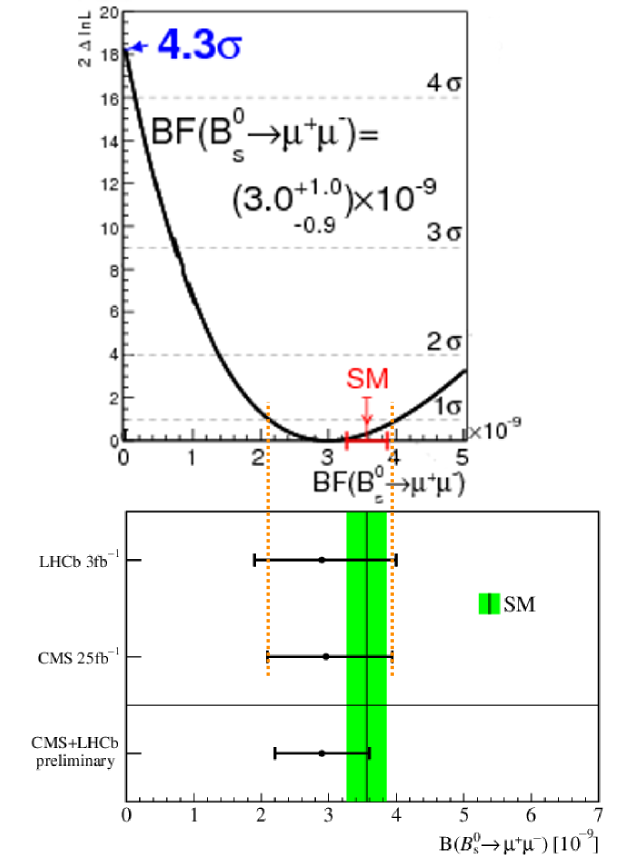
You’ll notice that the error bars on the combined result are smaller than those for either the CMS or LHCb results individually. That means the log-likelihood curve shoots up faster for the combined result, apparently fast enough that it’s above the \(5\sigma\) level by the time the branching ratio reaches zero — which is exactly the criterion to say the decay \(\mathrm{B}^0_s\to\ulp\ualp\) is officially discovered.

Of course, the standard model predicted that this decay would occur. So the thing that LHCb and CMS have discovered, namely that the log-likelihood is above the \(5\sigma\) level for a branching ratio of zero, isn’t really unexpected. What would be much more exciting is if they find that the log-likelihood is above the \(5\sigma\) level at the value predicted by the standard model — that would indicate that the real branching ratio is not what the standard model predicts, so some kind of new physics is definitely happening! But we’ll be waiting a long time to see whether that turns out to be the case.