Hooray, it’s time for science! For my long-overdue first science post of 2014, I’m starting a three-part series explaining the research paper my group recently published in Physical Review Letters. Our research concerns the structure of protons and atomic nuclei, so this post is going to be all about the framework physicists use to describe that structure. It’s partially based on an answer of mine at Physics Stack Exchange.

What’s in a proton?

Fundamentally, a proton is really made of quantum fields. Remember that. Any time you hear any other description of the composition of a proton, it’s just some approximation of the behavior of quantum fields in terms of something people are likely to be more familiar with. We need to do this because quantum fields behave in very nonintuitive ways, so if you’re not working with the full mathematical machinery of QCD (which is hard), you have to make some kind of simplified model to use as an analogy.

If you’re not familiar with the term, fields in physics are things which can be represented by a value associated with every point in space and time. In the simplest kind of field, a scalar field, the value is just a number. Think of it like this:

More complicated kinds of fields exist as well, where the value is something else. You could, in principle, have a fruit-valued field, that associates a fruit with every point in spacetime. In physics, you’d be more likely to encounter a vector-, spinor-, or tensor-valued field, but the details aren’t important. Just keep in mind that the value associated with a field at a certain point can be “strong,” meaning that the value differs from the “background” value by a lot, or “weak,” meaning that the value is close to the “background” value. When you have multiple fields, they can interact with each other, so that the different kinds of fields tend to be strong in the same place.

The tricky thing about quantum fields specifically (as opposed to non-quantum, or classical, fields) is that we can’t directly measure them, the way you would directly measure something like air temperature. You can’t stick a field-o-meter at some point inside a proton and see what the values of the fields are there. The only way to get any information about a quantum field is to expose it to some sort of external “influence” and see how it reacts — this is what physicists call “observing” the particle. For a proton, this means hitting it with another high-energy particle, called a probe, in a particle accelerator and seeing what comes out. Each collision acts something like an X-ray, exposing a cross-sectional view of the innards of the proton.

Because these are quantum fields, though, the outcome you get from each collision is actually random. Sometimes nothing happens. Sometimes you get a low-energy electron coming out, sometimes you get a high-energy pion, sometimes you get several things together, and so on. In order to make a coherent picture of the structure of a proton, you have to subject a large number of them to these collisions, find some way of organizing collisions according to how the proton behaves in each one, and accumulate a distribution of the results.

Classification of collisions

Imagine a slow collision between two protons, each of which has relatively little energy. They just deflect each other due to mutual electrical repulsion. (This is called elastic scattering.)

If we give the protons more energy, though, we can force them to actually hit each other, and then the individual particles within them, called partons, start interacting.

At higher energies, a proton-proton collision entails one of the partons in one proton interacting with one of the partons in the other proton. We characterize the collision by two variables — well, really three — which can be calculated from measurements made on the stuff that comes out:

• \(x_p\) is the fraction of the probe proton’s forward momentum that is carried by the probe parton
• \(x_t\) is the same, but for the target proton
• \(Q^2\) is roughly the square of the amount of transverse (sideways) momentum transferred between the two partons.

With only a small amount of total energy available, \(x_p\) and \(x_t\) can’t be particularly small. If they were, the interacting partons would have a small fraction of a small amount of energy, and the interaction products just wouldn’t be able to go anywhere after they hit. Also, \(Q^2\) tends to be small, because there’s not enough energy to give the interacting particles much of a transverse “kick.” You can actually write a mathematical relationship for this:

Collisions that occur in modern particle accelerators involve much more energy. There’s enough to allow partons with very small values of \(x_p\) (in the probe) or \(x_t\) (in the target) to participate in the collision and easily make it out to be detected. Or alternatively, there’s enough energy to allow the interacting partons to produce something with a large amount of transverse momentum. Accordingly, in these high-energy collisions we get a random distribution of all the combinations of \(x_p\), \(x_t\), and \(Q^2\) that satisfy the relationship above.

Proton structure

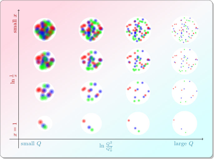
Over many years of operating particle accelerators, physicists have found that the behavior of the target proton depends only on \(x_t\) and \(Q^2\). In other words, targets in different collisions with the same values of \(x_t\) and \(Q^2\) behave pretty much the same way. While there are some subtle details, the results of these decades of experiments can be summarized like this: at smaller values of \(x_t\), the proton behaves like it has more constituent partons, and at larger values of \(Q^2\), it behaves like it has smaller constituents.

This diagram shows how a proton might appear in different kinds of collisions. The contents of each circle represents, roughly, a “snapshot” of how the proton might behave in a collision at the corresponding values of \(x\) and \(Q^2\).

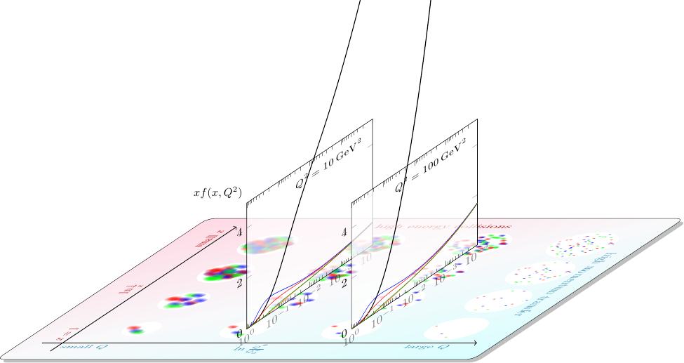
Physicists describe this apparently-changing composition using parton distribution functions, denoted \(f_i(x, Q^2)\), where \(i\) is the type of parton: up quark, antidown quark, gluon, etc. Mathematically inclined readers can roughly interpret the value of a parton distribution for a particular type of parton as the probability per unit \(x\) and per unit \(Q^2\) that the probe interacts with that type of parton with that amount of momentum.

This diagram shows how the parton distributions relate to the “snapshots” in my last picture:

The general field I work in is dedicated to determining these parton distribution functions as accurately as possible, over as wide of a range of \(x\) and \(Q^2\) as possible.

As particle accelerators get more and more powerful, we get to use them to explore more and more of this diagram. In particular, proton-ion collisions (which work more or less the same way) at the LHC cover a pretty large region of the diagram, as shown in this figure from a paper by Carlos Salgado:

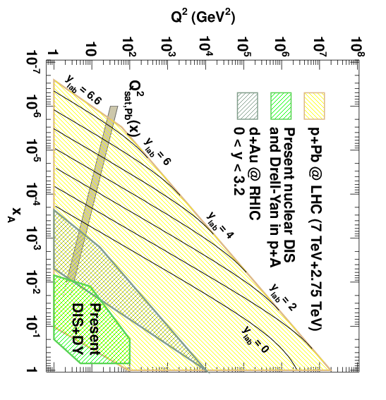
I rotated it 90 degrees so the orientation would match that of my earlier diagrams. The small-\(x\), low-\(Q^2\) region at the upper left is particularly interesting, because we expect the parton distributions to start behaving considerably differently in those kinds of collisions. New effects, called saturation effects, come into play that don’t occur anywhere else on the diagram. In my next post, I’ll explain what saturation is and why we expect it to happen. Stay tuned!