If you’ve been following the news about the discovery of the Higgs boson, you’ve probably noticed that it gets reported in two ways. There are the actual presentations with the full details of the experiments, which can only be understood by particle physicists their authors well, I’m assuming somebody knows what all of it means. Anyway, then there’s the other way. Sensationalized science journalism. “Hey, look, it’s a God Particle!!!11!” And Other Misrepresentations.

I think some of us want a middle ground, though. Certainly I would have, not too long ago. So if you’re not actually a physicist, but you’re also not afraid to look at a little math, this post is for you. (This is adapted from a post on Physics Stack Exchange.)

Spontaneous symmetry breaking

In order to understand the Higgs mechanism in detail, you need to know about two concepts that are involved in quantum field theory. The first is spontaneous symmetry breaking. This is actually a pretty simple idea: suppose that the physical laws that govern a system are symmetric in some way, meaning that you can make some kind of transformation on the system without changing the laws. That doesn’t necessarily mean the actual behavior of the system will be symmetric in the same way. The system might exist in a state that is affected by the transformation, even if the laws are not.

A common example is balancing a pencil on its tip. If you could get the pencil perfectly balanced, the system would be rotationally symmetric about its axis. Same goes for the physical laws that govern its behavior (gravity, Newton’s laws, etc.): if you rotate the whole setup around the pencil, nothing changes. However, realistically, the pencil is going to fall in some direction, and at that point the system is no longer rotationally symmetric. Once the pencil is rolling around on the table, if you rotate the whole setup around the tip of the pencil, something does change, namely the direction in which the pencil is pointing. Technically, the physical laws are still symmetric, but you don’t see the effects of that rotational symmetry anymore: now your pencil will roll off the table if you orient it in the wrong direction.

In its application to particle physics, spontaneous symmetry breaking occurs when there is some potential which has a local maximum that lies on the symmetry axis.

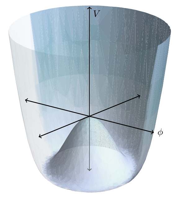
This is the famous “Mexican hat potential.” Mathematically, it’s represented by an expression of the form

In this expression, \(\mu\) and \(\lambda\) are constants and \(\phi\) is a quantum field. You can think of it as a complex-valued variable which is related to the quantum state at a point in spacetime. Now, for our purposes, the universe will “try” to “seek out” whatever state minimizes its potential, just like the balanced pencil will “seek out” the state that minimizes its potential. The only difference is that whereas the pencil changes its state by adjusting its position, the universe changes its state by adjusting the value of the field \(\phi\). Just as the pencil has to fall in some direction, the universe will have to experience a transition from its initial state on the peak in the center to some other state for which \(\phi\) lies at or near the bottom of the valley, having \(\abs{\phi} = \frac{\mu}{\lambda}\).

Local gauge invariance

The other concept involved is local gauge invariance. This one is a little harder to explain, because there’s no simple physical analogy, and it takes a fair amount of math.

Let me start with plain old invariance. This in itself is basically the same thing as symmetry: the idea that a physical theory doesn’t change under some sort of transformation. In the pencil example from above, the transformation was a physical rotation, which rearranges points in space. But you can also have a transformation that doesn’t affect points in space: in field theory, we have these fields which have associated values at every point in space, and a transformation could affect the values instead of the points. This is called a gauge transformation.

Gauge invariance means that you should be able to make gauge transformations to the fields involved in your theory without the physical laws changing as a result. An example of a gauge transformation is the phase rotation \(\phi(x)\to e^{i\alpha}\phi(x)\). It affects the value of a field at every point in space by multiplying it by a complex phase. If the parameter \(\alpha\) depends on spacetime position, \(\alpha(x)\), then we call it “local.”

Now to the technical part: explaining the significance of gauge invariance. Bear with me for a moment. In quantum field theory, there are basically two ways the fields themselves can show up: either directly, or as a derivative. They always show up in pairs or larger groupings, usually of a conjugate and a normal field, like \(\herm{\phi}\phi\). (\(\herm{\phi}\) is the Hermitian conjugate, which is the complex conjugate and transpose of a matrix-valued field.) Terms like that which involve only the fields themselves are automatically gauge invariant under phase rotation, because when you make the transformation, you get \(\herm{\phi}e^{-i\alpha(x)}e^{i\alpha(x)}\phi = \herm{\phi}\phi\); the phase factor just cancels out.

But when you have a term that involves derivatives, like \(\partial\herm{\phi}\partial\phi\) (where \(\partial = \frac{\partial}{\partial x}\)), called a kinetic term, you run into problems:

If you plug this into the gauge transformed kinetic term, \(\partial[e^{-i\alpha(x)}\herm{\phi}(x)]\partial[e^{i\alpha(x)}\phi(x)]\) (try expanding this for yourself), you’ll see that it will not simplify back to the original \(\partial\herm{\phi}(x)\partial\phi(x)\), because of those extra terms introduced by taking the derivative of \(e^{i\alpha(x)}\).

In order to keep local phase rotations from changing the physical laws, we need to modify the derivative. Instead of the plain old partial derivative \(\partial\), we’ll invent a new operator \(D\) so that the combination \(D\herm{\phi}(x)D\phi(x)\) is going to be gauge invariant. To do so, we add a connection \(A(x)\) to the derivative, turning it into the gauge covariant derivative

What makes this work is a stipulation that, as part of making a gauge transformation, the connection has to change too. For the example I’ve been using of a local phase rotation, the connection will need to change like this:

Essentially, making a gauge transformation not only alters the field, but also alters the operation of differentiation so that the combination of \(D\phi(x)\) doesn’t have any extra terms. Here’s how that works out: we start with

and make the gauge transformation, changing both \(A(x)\) and \(\phi(x)\),

A product rule and a bit of algebra gets you from there to

The first and last terms cancel out, and you’re left with

That means that the phase factor cancels out of \(D\herm{\phi} D\phi\), just as it did with the normal field terms. Cool!

Putting it all together

Where spontaneous symmetry breaking and local gauge invariance come together is in the Lagrangian. If you’re not familiar with what a Lagrangian is, you can kind of think of it as something like an energy density, but it’s not really that important. Just know that there are particular terms in it with particular meanings that I’ll identify as they come.

In real-world mechanical systems, the Lagrangian is formed by subtracting the potential energy from the kinetic energy. We can do the same thing in quantum field theory: form a Lagrangian by subtracting the potential \(V(\phi)\) from the kinetic term \(\frac{1}{2}D\phi^\dagger D\phi\). Hopefully this is starting to look familiar: I talked about a potential in the section on spontaneous symmetry breaking, and I talked about a kinetic term in the section on local gauge invariance. As the heading suggests, this is where it all comes together.

Most of quantum field theory is done perturbatively. This means we need the magnitude of the field (in this case \(\abs{\phi}\)) to be very small so that we can calculate interesting things as perturbation series, e.g. \(F(\phi) = F_0 + \phi F_1 + \cdots\). That would be all well and good if \(\phi\) were close to zero. But as I said in the section on spontaneous symmetry breaking, that’s typically not going to be the case. The universe will “seek out” the lowest potential, which means \(\abs{\phi}\) is going have a value closer to \(\frac{\mu}{\lambda}\), the minimum.

The solution? Just redefine the field. Instead of using \(\phi\), we’ll use \(\eta = \phi - \frac{\mu}{\lambda}\), which will be close to zero. \(\frac{\mu}{\lambda}\) is the vacuum expectation value of the field \(\phi\). So spontaneous symmetry breaking causes us to rewrite the Lagrangian as

It may seem like a pain, but seriously, you should work this out yourself. Plug the definition of \(\eta = \phi + \frac{\mu}{\lambda}\) into the original Lagrangian two equations up, expand out the terms, and see that it really does work out to this last expression. It’s just algebra, nothing too complicated, but there are a couple of neat cancellations that take place.

Now, as I said, I’m going to explain the meanings of some of the terms. In a QFT Lagrangian, there are three basic types:

• Kinetic terms involve derivatives of the fields. They are of the form \(D\herm{\eta}D\eta\), where \(\eta\) is a field. Loosely speaking, they represent the energy of motion of the field.
• Mass terms involve a product of the field and its conjugate, with some numerical coefficient. They are of the form \(M\herm{\eta}\eta\). The constant \(M\) is the mass of the particle that we associate with the field (although it takes a fair bit of calculation to show it).
• Interaction terms involve a product of three or more fields. They are of the form \(cA^2\eta\), where \(c\) is the coupling constant for the interaction. These terms represent fundamental interactions which are shown as individual vertices in Feynman diagrams. The term \(cA^2\eta\), for example, would represent an interaction between two \(A\) particles and one \(\eta\) particle.

Since we’re talking about the Higgs mechanism, the mass terms are of particular interest. Take a look at the two forms of the Lagrangian above. You’ll notice that both of them have a mass term for the field \(\eta\) (or \(\phi\)). But in the first expression, there is no mass term for the field \(A\), whereas in the second one, the mass term \(\frac{q^2\mu^2}{\lambda^2}A^2\) has “magically” appeared! Just because of what amounts to a change of coordinates, a seemingly massless particle turns out to have a mass! That is the Higgs mechanism in a nutshell.

In this example, \(\eta\) is the Higgs field, and \(A\) is a force carrier. It corresponds to the W and Z bosons which mediate the weak interaction. Notice that it’s actually the vacuum expectation value of the Higgs field, \(\frac{\mu}{\lambda}\), that gives the field \(A\) a mass. The terms which represent the Higgs boson, in particular its mass term \(-\mu^2\eta^2\) and its kinetic term, are separate from the term that grants mass to the field \(A\). So it’s not that the Higgs boson itself gives other particles masses; it’s a side effect of the mechanism as a whole.

If you’re curious for more detail about how all this works, I’d recommend a good textbook on particle physics and/or quantum field theory. At the introductory level, Griffiths is a good choice, but for the real details, look at something like Peskin & Schroeder or Halzen & Martin, which I’ve most directly based this analysis on.