The win-more effect of indirect elections

Posted by David Zaslavsky on November 6, 2012 11:16 AM

— Comments

It’s Election Day (in the US), and I have a relevant post I’ve been meaning to do for a while.

Suppose you have a binary experiment, one which has two possible outcomes with probabilities $p$ and $q = 1-p$. For example, voting. (Pretend there are only 2 parties) Overall, let’s say people vote Democrat with probability $p$ and Republican with probability $q$. Now suppose a large number $N$ of people all go out to vote; what can you say about the results?

In a statistical experiment like this, the possible results are drawn from a binomial distribution, in which the probability of getting $n$ Democratic votes (and $N - n$ Republican) is

$$P(n) = \binom{N}{n}p^n q^{N-n}$$

The probability that the Democrats will come out ahead is just the sum of all the probabilities for all the outcomes where $n$ is more than half of the total vote: we start at $n = \floor*{\frac{N}{2} + 1}$, which is the first integer greater than $\frac{N}{2}$, and add up probabilities all the way to $n = N$.

$$P_D(N,p) = \sum_{n=\floor*{N/2 + 1}}^{N}\binom{N}{n}p^n q^{N-n} = 1 - q^N (pq)^{\floor*{\frac{N}{2} + 1}}\binom{N}{\floor*{\frac{N}{2}+1}} {}_2F_1\left(\genfrac..{0pt}{}{1,\floor*{1 + \frac{N}{2}}-N}{2+\floor*{\frac{N}{2}}}\middle|-\frac{p}{q}\right)$$

Here ${}_2F_1$ is the ordinary hypergeometric function.

Well, huh. That’s kind of an ugly-looking expression. So let’s look at some pictures. Say you have $N=9$ people voting — an absurdly small country, for sure, but it’ll be a good example to see how the probabilities work out.

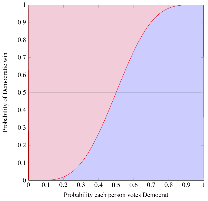
This graph shows the probability that the Democrat will win the election as a function of the probability that each of the 9 people will vote for him. For example, suppose you estimate, perhaps based on polling, that each person has a 40% chance of voting for the Democrat. (This is not quite the same as estimating that 40% of people will vote for the Democrat, but for much larger numbers of people, it’ll be close.) Look for 0.4 on the bottom axis of the graph, follow it up until you hit the red-blue boundary, and you find that you’re at about 27% on the vertical axis. So in this situation, the Democrat has a 27% chance of winning the election.

Let’s try another one. Same setup, but now with 99 people voting, not just 9.

You can immediately tell that this graph stays closer to 0 on the left and closer to 1 on the right, and is a lot steeper in the middle. When the graph does that, it means that the candidate who is favored to win, whichever one it is, is even more likely to win. In other words, a graph that stays close to 0 and 1 at the ends and has a steep slope in the middle indicates that the probability of an upset is very low.

For example, if you suppose each person has a 40% probability of voting for the Democrat, in this case that gives him only a 2% chance of winning — much less than the 27% in the 9-person election! This is what I call the “win-more effect”: even if a candidate has a tiny advantage in each individual person’s vote, when you put together a large number of people, that candidate will be overwhelmingly likely to win.

Take a look at one more fairly extreme case: $N=3000$, which is roughly the sample size used by some public opinion polls. (Don’t quote me on that, I’m not positive.)

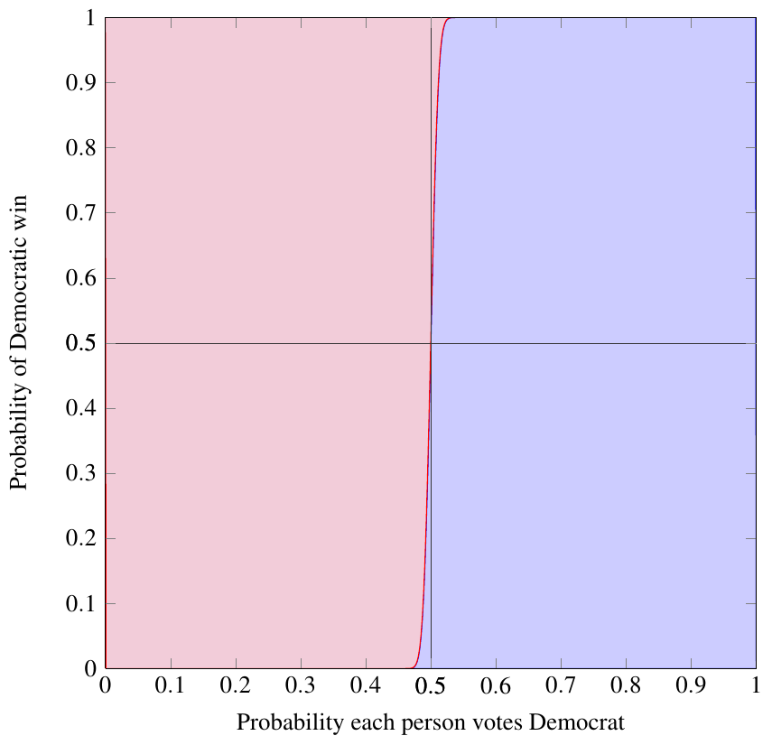
Here the slope in the middle is almost vertical. A candidate who has a 40% chance of winning any individual vote has essentially zero chance of winning the overall election. But it’s not perfectly vertical; if the race is close, like 49% to 51%, the losing candidate still has a 13% chance to pull off an upset! The win-more effect “ramps up” very quickly for small numbers of people, but very slowly for larger numbers, so that if a race is very close in the popular vote, it can still be competitive even for a huge voting population.

Indirect elections

Of course, in the United States, our presidential election is more complicated than that. We don’t vote directly for the president; instead we choose electors who will go on to cast the actual votes. This is called an indirect election, and it modifies the effectiveness of the win-more effect — but perhaps not in the way you’d think!

Let me go back to that first example with 9 people in the election. But this time, suppose the 9 people are just the population of one of several states in a larger country. To make the numbers work out, I’ll say there are 11 states, each with 9 residents, for a total of 99 people.

Hopefully it’s clear that if these 99 people in 11 states are choosing a president using an indirect election (like the US electoral college), the graph I made above for the 99-person election doesn’t necessarily apply anymore. What we need to do this time is think of the election in two stages:

First, there are 11 individual elections with 9 voters each. I’ve already crunched the numbers and shown the graph for an election of 9 voters, and for any given probability $p$ that an individual voter will choose the Democrat, we can calculate the probability $P_D(9,p)$ that any one state of 9 people will go to the Democratic candidate. ($P_D$ is the ugly function I derived at the top of this post, the same one plotted in the graphs above.)
The second level is effectively another election where the states are the voters. In this second-level election, there are 11 participants, and for each one the probability of casting a Democratic vote is $P_D(9,p)$, just the output probability from the first step. So the overall probability of a Democratic candidate winning is $P_D(11,P_D(9,p))$.

Naturally, I can also do the analogous calculation for the probability of a Republican winning, and I’d get $P_R(11,P_R(9,p))$. These had better add up to 1 if the calculation is to make sense. And they do:

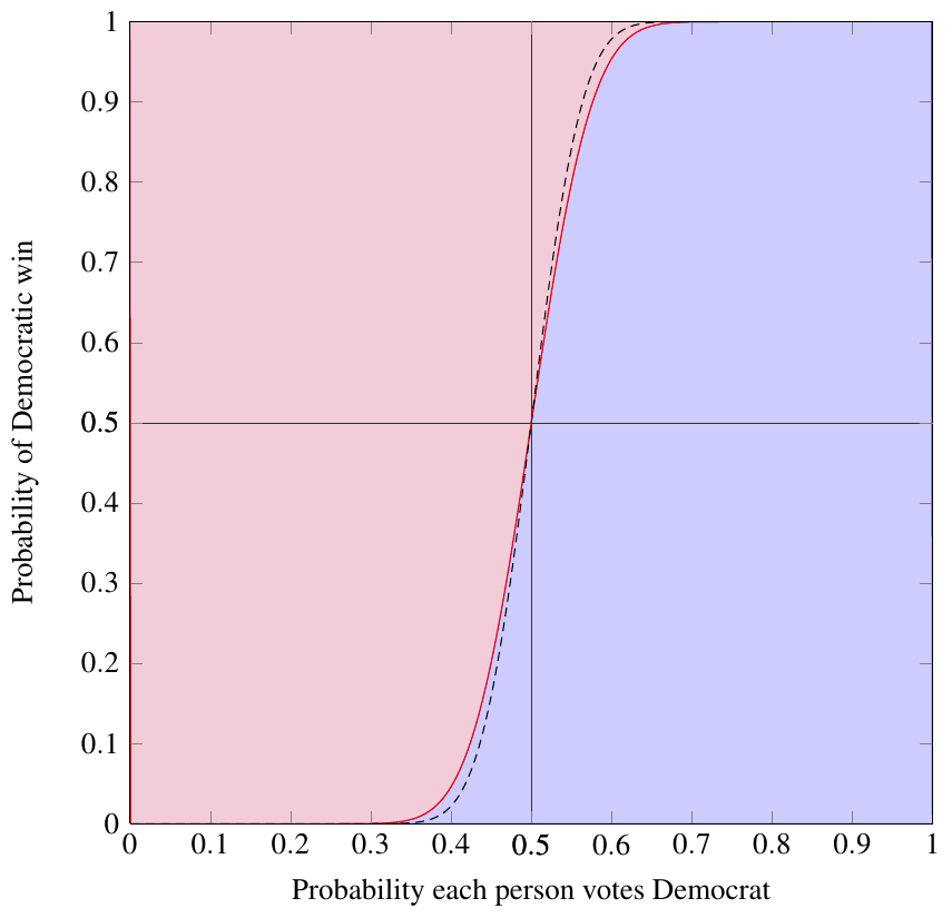
Probabilities for an 11x9 indirect election

Now this is an interesting result! Let’s look at how the graph for the indirect election, the red-blue boundary, compares to the graph for the 99-person direct election, which I’ve added in as a dashed black line. The curve for the indirect election is less steeply sloped near the center, which means the win-more effect is less prevalent in this indirect election: having an upset is actually more likely! For example, if people have a 40% chance to vote for the Democratic candidate, that gives him a 2.2% chance of winning in a direct election but a 4.6% chance of winning an indirect election, more than twice as likely.

Honestly, that’s not what I expected to find.

I know it’s not really well justified to extend this conclusion to real elections, because there are so many differences and complications in a real election that I haven’t accounted for: the states are different sizes, different people have different probabilities of voting one way or another, in fact you can’t even measure those probabilities in many cases… but I feel like the general conclusion, that indirect elections temper the win-more effect, should be relevant. If it is, we’d expect to see that the results of the electoral college vote are statistically closer than the results of the popular vote, in some sense. I’m not quite sure how you would do the analysis to figure out whether that’s correct, but maybe that’s best left for next year.

Right now, it’s time for me to head off to the polls. FOR SCIENCE!