It’s been far too long since I posted anything — almost three weeks, in fact, since the end of NaBloWriMo. So I took the time to make a solid writeup of the speculation that we may be living in a computer. Consider it my Christmas present to the blogosphere. Happy holidays everyone!

Have you ever wondered if everything you know might only exist inside some hyperintelligent alien’s computer?

It’s a fun possibility to consider, that we might be living in a computer simulation, and we might even be able to figure out how to manipulate it. It even makes for some great science fiction (as well as some terrible science fiction :-P perhaps). But in reality, figuring out whether the universe is a simulation isn’t as easy as popping a red pill and waking up in an alternate reality with one less layer of abstraction. If we are in a simulation, the way it’s going to reveal itself is in the tiny details of physical processes that take place on sub-subatomic distance scales.

There is actually a branch of physics, lattice QCD, that is entirely devoted to simulating reality. Right now it only works for very small volumes, barely large enough to fit a proton, but that’s already enough to give us a sense of what kinds of tiny details, or artifacts, can prevent a simulation from being completely accurate. These artifacts are the subject of a recent paper by Silas Beane, Zohreh Davoudi, and Martin Savage. It’s a nice concise piece of work: they imagine that the universe is a computer simulation on a cubic grid, similar to simple lattice QCD models, and just calculate some of the observable consequences of this grid.

Unfortunately, when this hit the popular press (and the blogosphere), everything went to hell. Nearly every time I’ve seen this research reported, it completely misrepresents the original paper. People have been saying everything from that the scientists are proposing a test for whether the universe is a simulation, to that they’ve actually shown that it is. But none of that is true! To clear things up, I wanted to examine the paper itself, and clear up what exactly these physicists did conclude.

Fields on a grid

I’ll start with a primer on how a simulation on a grid works. The grid itself is just a set of points in space (or spacetime) that you’re going to include in your simulation. Generically, you can pick the points any way you want, but the simplest way, and the one discussed in the BDS paper, is to just pick them evenly spaced in every dimension. The distance between adjacent points in each dimension is the grid spacing, and the smaller that is, the more accurate the simulation will be.

On the grid, you have some number of fields. Normally a field is a thing that has a value at every point in space. But when you’re working on a grid, the points that are part of the grid are effectively the only points in space. So your simulated fields have values at every point on the grid. In reality, if you weren’t doing a simulation, the fields would also have values at points between the grid points, but for the simulation, you have to ignore that and hope the field doesn’t do anything too weird in the spaces.

Once you have the grid (the points in spacetime) and the fields (the values at those points), the actual process of simulation is simple, in principle. At each time step, you go through each point on the grid and use some set of rules to calculate new values for the next time step. The particular set of rules you use depends on what physical system you’re trying to simulate. If it’s a weather simulation, you would use some discrete approximation of the laws of fluid dynamics. If it’s a cosmological simulation, you would use some discrete approximation of general relativity. And if you’re trying to simulate the structure of a proton, as they do in lattice QCD, you would use some discrete approximation of the laws of quantum chromodynamics. The point is, when you’re doing a simulation on a grid, you always need a discrete approximation of the physical laws that govern your system — you have to use modified laws that only use the points on your grid, not the nonexistent (in your simulation) points in between. And that’s the inherent limitation of any grid simulation: you have to ignore the fine details of the behavior of the fields between grid points. It’s those fine details that cause the slight differences that would expose a grid simulation as a simulation.

Details of the grid model

Now let’s turn to the actual paper. Beane, Davoudi, and Savage started with the quantum electrodynamic description of a charged particle in an EM field, which in our ordinary, continuous reality is given by this expression, the Lagrangian density:

The details of what this expression means don’t really matter. But since I know some of my readers who don’t know quantum field theory won’t be happy unless they can make some sense of it:

• \(\psi\) is the charged particle field — let’s say it’s the electron
• \(m\) is the charged particle’s (electron’s) mass
• \(q\) is the particle’s charge, which also determines how strongly the charged particle and the EM field interact
• \(A_\mu\) is the electromagnetic vector potential

So for example, the term \(iq\bar\psi\gamma^\mu A_\mu\psi\) represents an electron (\(\psi\)) interacting with the electromagnetic field (\(A_\mu\)). It’s that term that determines how electrons react to electromagnetic forces. But like I said, most of that doesn’t really matter.

What does matter is how you have to modify that expression to make it work on a grid. The modified expression looks like this:

where \(b\) is the grid spacing, \(F^{\mu\nu}\) is a function of the electromagnetic vector potential, and \(\mathcal{C}_p \approx 1\) and \(\sigma_{\mu\nu}\) are basically constant coefficients. The most important change is that we have a new term, \(\mathcal{C}_p\frac{qb}{4}\bar\psi\sigma_{\mu\nu}F^{\mu\nu}\psi\), which involves an additional, different interaction between electrons and the electromagnetic field! This is an example of a simulation artifact. It modifies the way in which electrons respond to EM fields, and so it could have observable consequences.

What could we see?

In the rest of the paper, the scientists identify three ways in which this particular simulation artifact could show itself, if it really exists. Before we get into that, though, it’s important to pause and remember what we’re dealing with here: this is a toy model. It’s only the very simplest way in which one aspect of the universe (i.e. the electromagnetic force) could be simulated, and bear in mind that we don’t even have any reason to believe the universe is a simulation! Nobody honestly expects this model to be real, it’s only meant to show how these kinds of calculations could work.

OK, now that that’s out of the way, what did they find?

Modified muon magnetic moment

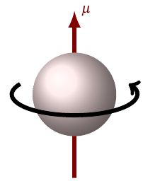An electron or muon, because it has charge and angular momentum, acts like a magnet. In physics terms, it has a magnetic dipole moment \(\mu\). The magnitude of this dipole moment — the strength of the magnet — is expressed as

where \(\mu_B\) is a fixed physical constant, the Bohr magneton, and \(g\) is a number which depends on the particle: \(g_e\) for the electron, \(g_\mu\) for the muon. You can think of \(g\) as measuring the electron’s or muon’s magnetic moment in units of \(\frac{\mu_B}{2}\). This number has been measured very precisely and also can be predicted very precisely from QED; in fact, the measurement of \(g_e\) is the most precisely confirmed prediction in all of physics!

If the extra “grid term” from the Lagrangian density were real, it would modify the above equation to

In this case, QED still predicts the value of \(g\), but when we think we’re measuring \(g\), we would actually be measuring \(g + \frac{2c}{\hbar}mb\mathcal{C}_p + \orderof{b^2}\). That means, if this theory were true, the measured and calculated values of \(g\) should differ by \(\frac{2c}{\hbar}mb\mathcal{C}_p\). It just so happens that a slight difference of this type does exist for \(g_\mu\): its measured value is \(-2.00233184178\pm 0.00000000087\), whereas the QED prediction is \(-2.00233183604\pm 0.00000000070\). That’s a difference of \((5.72\pm 1.57)\times 10^{-9}\), and if you set that equal to \(\frac{2c}{\hbar}m_\mu b\mathcal{C}_p\), it tells you how big the grid spacing \(b\) would have to be to account for that difference:

(There are some subtleties I’m glossing over here, but that’s the gist.) So if the universe is a simulation on a cubic grid, the spacing can’t be any bigger than that, otherwise our measurement of the muon magnetic moment would be even more different from the QED prediction than it is. Effectively, we have an upper bound on the grid spacing — one that we’re still (un)comfortably far away from being able to see directly. But nothing prevents the grid spacing from being smaller, or nonexistent; it’s entirely possible that the difference between the measured and predicted magnetic moments is due to something else entirely.

Rydberg constant

The Rydberg constant \(R_\infty\) is the amount of energy it takes to break apart a hydrogen atom into a free proton and a free electron. This amount of energy can be fairly precisely measured, and then we can work backwards from that value to get a value for \(\alpha\), the electromagnetic coupling. (It’s related to the electron’s charge by \(\alpha = \frac{q^2}{4\pi\epsilon_0\hbar c}\); either one of those variables, \(\alpha\) or \(q\), can be used to represent how strongly electrons interact with EM fields.)

We can also get a value for \(\alpha\) from the electron’s magnetic moment. But it turns out that, if we live in a simulation on a cubic grid, what we measure using the Rydberg constant method and what we measure using the magnetic moment method aren’t quite the same thing! The difference between those two measurements is related to the grid spacing \(b\).

Unfortunately the paper is pretty light on details when it comes to this method, so there’s not much I can say, but I can give the punch line: the difference between the two measured values of \(\alpha\) is \((1.86\pm 5.51)\times 10^{-12}\). That’s actually consistent with zero: it seems entirely likely that there is no difference at all, which is exactly what we’d expect to see for a fully continuous, non-simulated universe.

Cosmic ray cutoff

Cosmic rays are pretty much what they sound like, except that they’re not exactly rays. They’re PARTICLES FROM SPACE!!!! And some of them have very high energies, many orders of magnitude more than what we can produce in any particle accelerator on Earth (like the LHC).

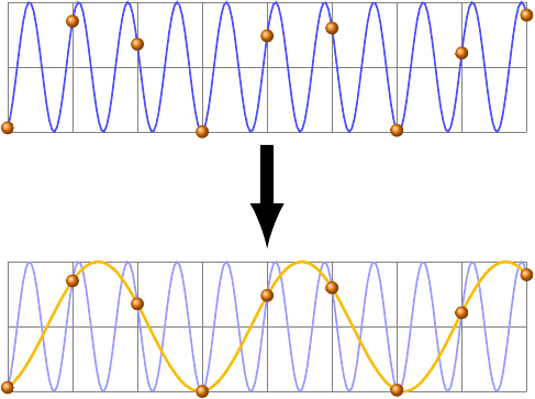
It turns out, though, that ultra-high-energy particles, specifically those with energy higher than about \(\frac{hc}{2b}\), cannot exist on a cubic grid! That’s because of an effect called aliasing, which will be familiar to anyone who’s worked with sound engineering or digital signal processing. Aliasing basically means that any wave with a wavelength smaller than twice the grid spacing behaves exactly like a different wave with a wavelength larger than twice the grid spacing, like the blue wave and the orange wave in this picture.

And since wavelength is inversely proportional to energy for a massless particle, \(E = \frac{hc}{\lambda}\), along each of the grid axes there is an upper limit of \(\frac{hc}{2b}\) on the energies of waves that can be simulated. As long as you’re talking about particles whose masses can be neglected (which is definitely true for these ultra-high-energy cosmic rays), no individual object in the simulation can ever act like it has any more energy than \(\frac{hc}{2b}\). (This limit is the spatial equivalent of the Nyquist frequency in signal processing.)

If we’re going to consider the possibility that the universe is a simulation, this energy limit that comes from aliasing has to compete with a different energy limit, the GZK cutoff, which arises from an entirely different reason. According to special relativity, a cosmic ray proton with more than a certain energy (\(\SI{5e19}{eV}\)) can collide with a photon from the cosmic microwave background with enough energy to decay into a pion and a slower proton. These CMB photons are everywhere — they quite literally permeate all of space — and so any cosmic ray with enough energy almost certainly will collide with one of them, and will be stopped long before it gets to Earth.

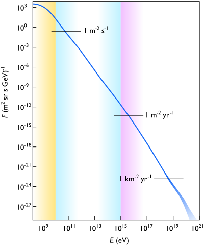The reason for that value of \(\SI{5e19}{eV}\) is clearest if you think about a collision between a proton and a CMB photon from the proton’s perspective. It sees a highly blueshifted CMB: instead of a uniform thermal distribution of photons with energies corresponding to the temperature of the universe, \(\SI{2.73}{K}\), it sees photons coming from one direction with much higher energies. If the proton is moving fast enough, it sees those photons coming with enough energy to excite the proton and turn it into a delta baryon, which then emits a pion to decay into a slower-moving proton. In this way, an energetic proton will repeatedly lose energy until it slows down enough that it doesn’t interact with the CMB anymore. The end result is that cosmic rays with energies more than the GZK cutoff should be quite rare. And in fact they are: recent observations by the Auger and HiRes cosmic ray telescopes, among others, do actually see many fewer cosmic rays than expected with energies above \(\SI{5e19}{eV}\).

So in a universe simulated on a cubic grid, we have two different cutoffs that limit the number of cosmic rays above a certain energy: the GZK cutoff, which kicks in at \(\SI{5e19}{eV}\), and the grid cutoff, which kicks in at the unknown value \(\frac{hc}{2b}\). Depending on the value of \(b\), there are three (but really two) possibilities:

• \(\frac{hc}{2b} < \SI{5e19}{eV}\): the grid cutoff is less than the GZK cutoff. In this case there are no cosmic rays with high enough energies to see the GZK cutoff at all. This is clearly not true in our universe because, as I mentioned, various telescopes have actually seen those high-energy cosmic rays.
• \(\frac{hc}{2b} \gg \SI{5e19}{eV}\): the grid cutoff is greater than the GZK cutoff. In this case there are few to no cosmic rays with high enough energies to see the grid cutoff. This could conceivably be true in our universe, if you accept the idea that the universe might be a simulation on a cubic grid. If you solve the inequality for \(b\), you get an upper limit of \(b \ll \frac{hc}{2(\SI{5e19}{eV})} \lesssim \SI{1.2e-24}{m}\).
• \(\frac{hc}{2b} \approx \SI{5e19}{eV}\): the grid cutoff and the GZK cutoff are about equal. This case is actually going to look similar to the last one, and also similar to what we would see if there is no grid cutoff at all, because in each one we just see a dropoff in the number of cosmic rays above \(\SI{5e19}{eV}\). However, there is one key feature that sets this option apart from the others: the grid cutoff is different in different directions! In the lingo of physics, we say the grid cutoff is not rotationally invariant; in the language of astrophysics, we say it’s anisotropic. Hopefully it’s intuitively clear why this would be true: the spacing between points on the grid is different if you’re moving along the direction of an axis as opposed to if you’re moving diagonally. And that means that the grid cutoff will behave differently depending on which direction a particle is moving relative to the grid. If we actually live in this kind of simulation, then, we can expect to see the highest energy particles traveling only in certain directions in space.

If we were to actually observe a directional distribution of these ultra-high-energy cosmic rays, that would be huge. Nearly all of modern physics is based in part on the principle of rotational invariance, which means that fundamentally, there are no special directions. If we saw high energy cosmic rays traveling only along the axes of a cube, that would blow that out the window, and suddenly we’d have to take a whole new look at the physics of high energy particles! It wouldn’t change anything in our everyday lives, but it would be really cool.

But of course, no sign of any of this has ever been observed. And judging by the results presented in this paper, we’re a long way away from finding any simulation artifacts, even if they do exist. So for the foreseeable future, the continuum of reality remains just that.