Hooray, it’s time for another blog post! What I’m writing about this time is kind of old news — and don’t worry, there’s more to come on just why I haven’t been able to write about it for so long — but very interesting nonetheless.

A few weeks ago, two separate physics experiments announced that they had discovered a tetraquark, a composite particle made of four quarks. Or rather, that’s what all the popular news coverage said. But what really happened? The discovery of a real tetraquark would be huge news, so I’m sure not going to trust the media reports on this one. As always, I’m going straight to the source: the original papers by the BES III and Belle collaborations.

Two or Three is Company, Four’s a Crowd

Before delving into the discovery itself, I’m going to tackle the burning question on everybody’s mind: what’s so special about a particle made of four quarks?

To understand that, we have to look to quantum chromodynamics (QCD), the theory of how “color-charged” particles interact. In some ways, QCD is superficially similar to quantum electrodynamics, the theory of how electrically charged particles interact. You can rely on your familiar intuition that positive and negative charges attract, for instance. Just as positively charged protons and negatively charged electrons attract each other, and can bind together to form atoms, particles with matching postive and negative color charges can bind together to form particles with two quarks (actually one quark and one antiquark) which are called mesons.

But unlike electromagnetism, where there is only one kind of charge (electric), QCD includes three kinds of charge, each of which can be independently positive or negative. The three charges are called red, green, and blue, even though they have nothing to do with visible colors. They’re often shown in a diagram like this one:

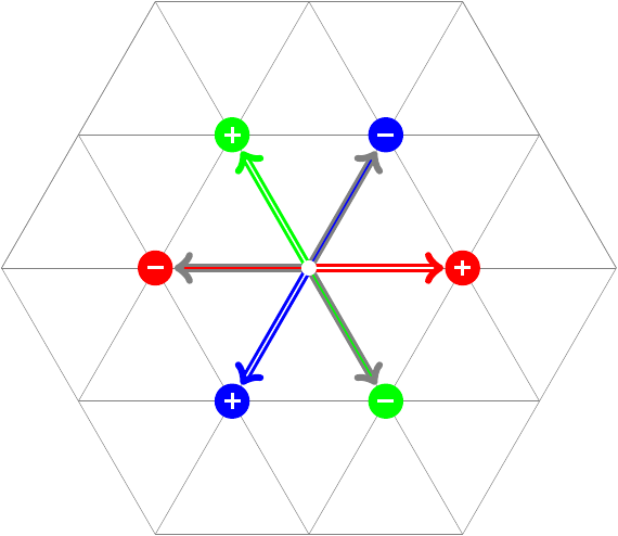
If there are three independent charges, why don’t I show them using three dimensions? Well, it turns out that a combination of a red, a green, and a blue charge is precisely equivalent to no color charge at all. Accordingly, if you add together the (positive) red, green, and blue vectors from that image, it gets you right back to the center. An object like this — whether uncharged, or positive and negative of the same color, or red+green+blue, or some combination of those — is called a color singlet.

Now, one of the consequences of QCD, and a rule drilled into all young particle physicists at an early age, is that all naturally occurring particles are color singlets. The reason is simple: remember that the force which acts on color-charged objects (analogous to how the electromagnetic force acts on electrically charged objects) is called the strong force, because, well, it’s strong. If there were any loose color-charged particles floating around, they would be immediately attracted to other particles with different color charges, forming color-neutral groups. In fact this process, hadronization, actually took place early in the universe’s formation, shortly after the big bang. It also happens in heavy-ion collisions in modern particle accelerators, anywhere a quark-gluon plasma is produced.

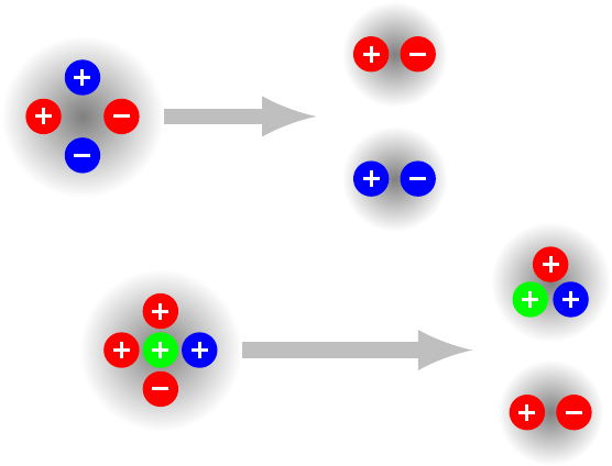
There are plenty of known particles that constitute the simplest kinds of color singlets: a quark and antiquark of the same color or three quarks (or antiquarks) of different colors. But what about more complicated combinations? You can imagine a particle composed of two quarks and their corresponding antiquarks (a tetraquark) or four quarks and an antiquark, or vice-versa (a pentaquark). They’re valid color singlets because the net color charge is zero, but they can break apart into smaller color singlets with two or three quarks, and that’s presumably why there aren’t a bunch of them floating around the universe.

Like other unstable particles, though, tetraquarks and pentaquarks can be produced in the collisions made in a particle accelerator. At least, that’s what the theory says, but in decades of colliding particles (until about a year ago, if this discovery is real), we’ve never seen clear evidence that a tetraquark or pentaquark has ever been produced.

Finding a Particle in a Haystack

If you have a particle that decays into two other particles, the total momentum of the two products, or final-state particles, is equal to the momentum of the original, initial-state particle. Same goes for energy.

This is useful because special relativity tells us the energy and momentum of the original particle satisfy \(E_i^2 - p_i^2 c^2 = m_i^2 c^4\), where \(m_i\), the mass of the particle, is a constant. Plugging in, you get

All these variables, the energies and momenta of the products, are measured by the detector. You can plug the energies and momenta of pairs of particles into this formula, and if they came from the same decay, you’ll get the mass of the intermediate particle they came from. If they didn’t come from the same decay, you’ll get a more or less random value.

Somewhat confusingly, \(m_i\), also denoted \(m_{12}\), is called the invariant mass of the pair 1,2 even if it doesn’t match the mass of the thing the particles decayed from (or even if those two particles didn’t come from the same decay at all).

Virtual particles

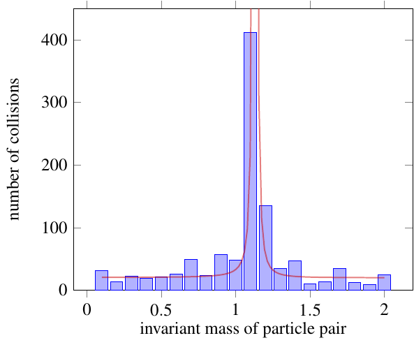
Hold on — I lied. Yes, just like everything else in physics, it’s not that simple. In quantum field theory, a particle — which is really a certain kind of disturbance in a quantum field — doesn’t satisfy \(E_i^2 - p_i^2 c^2 = m_i^2 c^4\) exactly. If you produce a bunch of identical particles of a type that has mass \(m_i\), the quantity \(E_i^2 - p_i^2 c^2\) won’t always be equal to \(m_i^2 c^4\); instead, it follows a probability distribution which roughly resembles

When you take pairs of particles and calculate \((E_1 + E_2)^2 - (\vec{p}_1 + \vec{p}_2)^2 c^2 = m_{12}^2 c^4\) (and note that \(m_{12}\) is still called the invariant mass of the pair despite being almost completely unrelated to the mass of any particle involved), even if they did come from the same decay, you don’t get a single value. You get a peaked distribution, like this:

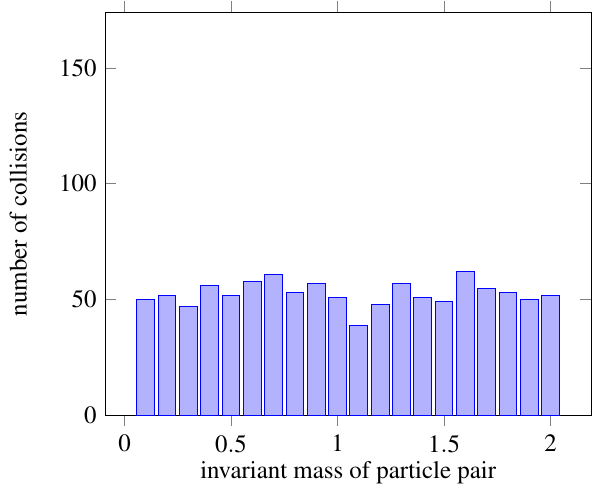
Particles which didn’t come from a single decay will still give you a mostly flat distribution:

Dalitz plots

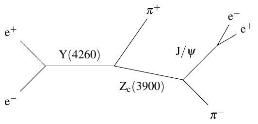
In electron-positron collisions, the kind that take place in BES III and Belle, the only way you get exactly two final-state particles out of the collision is if the electron and positron turn into a single particle which then decays into two products. There are not a whole lot of options for what that single particle can be, because of all the conservation laws that apply; it’s basically limited to photons, Z bosons, and Higgs bosons. So to have any hope of finding other interesting particles, we have to look at other collisions with more complicated decay chains. For example, the tetraquark candidate that BES III and Belle have discovered, called the \(Z_c(3900)\), is produced like this:

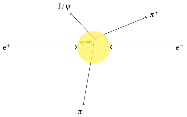
A multi-stage decay means that more than two particles are produced, and that means you can’t just pick the two decay products of the particle you want to discover. Think about it — if everything in the yellow circle below is hidden from you, how would you know that it’s the \(J/\psi\) and \(\pi^+\) that came from the \(Z_c(3900)\), rather than the \(J/\psi\) and \(\pi^-\)?

In these cases, the way to go is make histograms of \((E_1 + E_2)^2 - (p_1 + p_2)^2 c^2\), like those in the last section, for each pair of particles that comes out. If any two of those particles came from one decay, you’ll get a spike in the corresponding plot, but the other plots will be basically flat.

However, if there are only three final-state particles, as in \(\elp\ealp\to J/\psi\pipm\pimm\), we don’t actually need to make all three histograms. Check this out:

The analogous equation works for momentum as well:

Subtracting \(c^2\) times the latter equation from the former, since \(E^2 - p^2 c^2 = m^2 c^4\), gives

(with an overall factor of \(c^4\) that I left out). Now, \(m_{J/\psi\pipm\pimm}\) on the left is the same as the center-of-mass energy of the colliding electron and positron. And the masses of the individual particles are known, so the three quantities we’d be making histograms of, \(m_{J/\psi\pipm}^2\), \(m_{J/\psi\pimm}^2\), and \(m_{\pipm\pimm}^2\), always have to add up to the same value! They’re not independent. That means any peak from an intermediate decay has to show up on at least two of the plots.

With that in mind, you can put two of these histograms — any two — on the two axes of a scatter plot. This is called a Dalitz plot. Each \(\elp\ealp\to J/\psi\pipm\pimm\) collision appears as one point on the graph, with x coordinate \(m_{J/\psi\pipm}^2 c^4 = (E_{J/\psi} + E_{\pipm})^2 - (\vec{p}_{J/\psi} + \vec{p}_{\pipm})^2 c^2\) and y coordinate \(m_{J/\psi\pimm}^2 c^4 = (E_{J/\psi} + E_{\pimm})^2 - (\vec{p}_{J/\psi} + \vec{p}_{\pimm})^2 c^2\). An intermediate particle will show up as a clumping together of points along either the horizontal or vertical axis, corresponding to a peak in a histogram.

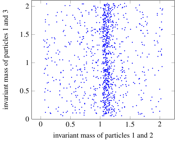
This example uses the same data from the histograms in the previous section. It’s much cleaner than you’d get in reality, but you see the point: the peak of the histogram corresponds to the dense line of dots running up and down the middle of the plot.

The Big Deal… Maybe

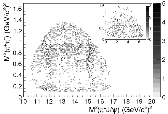
For the real data, we turn to the papers from BES III and Belle. Both experiments have published Dalitz plots showing \(M_{J/\psi\pipm}^2\) against \(M_{\pipm\pimm}^2\). This is from BES III:

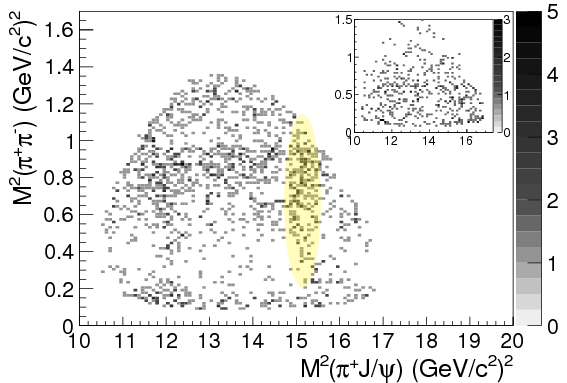
and this from Belle:

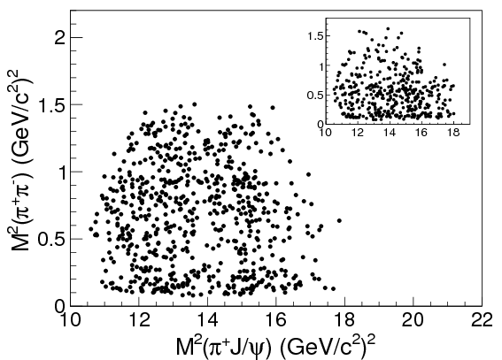
The inset plots in the top right show an estimate of the background, based on the “\(J/\psi\) sideband”: essentially, collisions in which no \(J/\psi\) was produced.

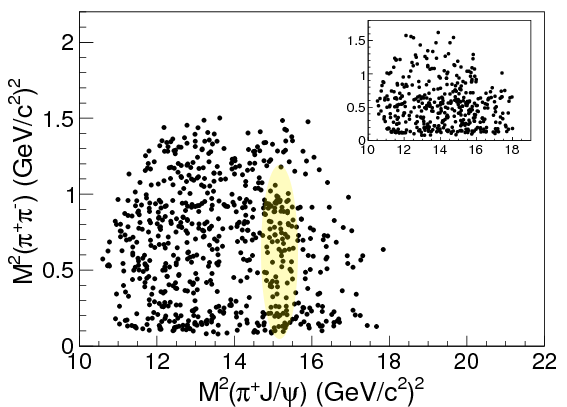
If you look around \(M_{J/\psi\pi^{\pm}}^2 = \SI{15.2}{GeV^2}/c^4 = (\SI{3.9}{GeV}/c^2)^2\), you can see a slight clump of points running up and down the graph. Here it is highlighted for clarity: BES III

and Belle

It’s not all that clear in these plots, but if you look at the corresponding 1D histograms for \(M_{J/\psi\pipm}\) (formed by adding up dots down the columns), there’s a clear difference between the theoretical prediction without the particle (red lines) and the data (black dots):

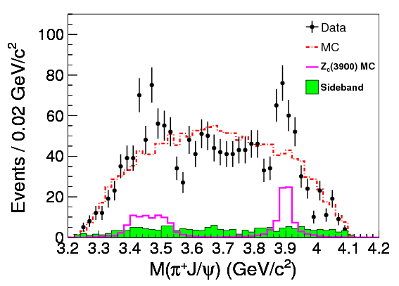
(BES III)

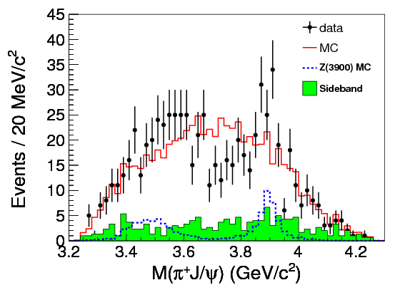
(Belle). You can see the spike at \(\SI{3.9}{GeV}/c^2\), and another bump at \(\SI{3.5}{GeV}/c^2\) which the paper assures us is an “echo” of the same particle. That structure indicates an intermediate particle, the \(Z_c(3900)\), with a mass of around \(\SI{3.9}{GeV}/c^2\) (the peak of the graph), which decays into a \(J/\psi\) and a \(\pipm\).

That’s the funny thing, though. Since the \(J/\psi\) is electrically neutral and the pion has an electric charge of +1, we know the \(Z_c(3900)\) also has +1 electric charge. On the other hand, the \(J/\psi\) is made of a charm quark and anticharm quark, which means that most likely the \(Z_c(3900)\) also contains charm and anticharm quarks. That combination is electrically neutral. So if \(Z_c(3900)\) has charm and anticharm quarks, it must also have some other combination of quarks with an electrical charge of +1. That takes at least two additional quarks, for a total of four or more.

When a Tetraquark Isn’t Really a Tetraquark

The mere fact that the \(Z_c(3900)\) seems to contain at least four quarks doesn’t necessarily make it a “true” tetraquark, though. In other words, we don’t know that it’s actually a single particle. It could be a bound state of two mesons made of two quarks each, a meson molecule, which would be interesting, but not as exotic and exciting as a single particle made of four quarks.

The difference between these two options is kind of subtle. Try this analogy on for size: think of it like two balls of slightly dry clay. If you take the two balls and stick them to each other, you’ll get what could reasonably be called one lump of clay, but if you then pull this new lump apart, it’ll split back into the two original balls, more or less. That’s because the chemical bonds between the clay from one lump and the clay from the other lump aren’t quite as strong as the bonds holding each lump of clay together. On the other hand, if you push the balls together hard, and knead them around a bit, now you’ve got a bona fide single lump of clay. You can pull it apart into two pieces, sure, but the clay from both original balls is all mixed up, so you’re not going to split it the same way it was originally split. There isn’t one easy division for the clay like there was when you had two separate balls stuck together.

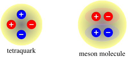
Mesons and tetraquarks work kind of like that. If you have a molecule of two mesons, in each meson, the quark and antiquark are bound together tightly, like the clay in one lump. The binding between one meson and the other will be a little weaker. But with a “true” tetraquark, all four quarks are equally well bound to each other, forming one object, like when you knead all the clay together. Right now, we can’t tell these two options apart, so the \(Z_c(3900)\) could be either (or something else entirely). It should be possible in principle to distinguish between them based on how quickly and how often the \(Z_c(3900)\) decays into various other types of particles, but we’re going to need much more precise measurements to make that happen. This is definitely something to keep an eye out for in future results from both BES III and Belle!