A simple regularization example

Posted by David Zaslavsky on November 20, 2012 3:00 AM

— Comments

Earlier this month I promised to show you a simple example of regularization. Well, here it is. This is a particular combination of integrals I’ve been working with a lot lately:

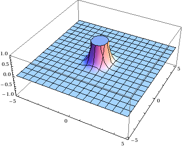
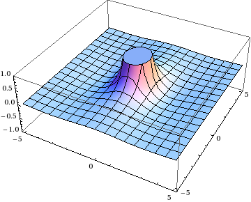
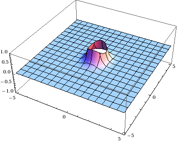
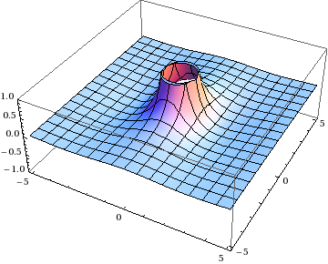
$$\iint_{\mathbb{R}^2} \uddc\mathbf{x}\frac{e^{-x^2}}{x^2}e^{-i\mathbf{k}\cdot\mathbf{x}} - \iint_{\mathbb{R}^2} \frac{\uddc\mathbf{y}}{y^2}e^{-i\xi\mathbf{k}\cdot\mathbf{y}}$$

A quick look at the formulas shows you that both integrands have singularities at $\mathbf{x} = 0$ and $\mathbf{y} = 0$.

OK, well, that’s why we have two integrands. We can change variables from $\xi\mathbf{y}\to\mathbf{x}$, subtract them, and the singularities will cancel out, right? You can do this integral by hand in polar coordinates, or just pop it into Mathematica:

$$\iint_{\mathbb{R}^2} \uddc\mathbf{x}\frac{e^{-x^2} - 1}{x^2}e^{-i\mathbf{k}\cdot\mathbf{x}} = -\pi\Gamma\biggl(0, \frac{k^2}{4}\biggr)$$

Just one problem: that’s not the right answer! You can tell because the value of this integral had better depend on $\xi$, but this expression doesn’t. This isn’t anything so mundane as a bug in Mathematica. It’s a “bug” in math itself.

See, when you have an undefined quantity, like a divergent integral, you can’t just keep doing math with the expression that represents it. That can lead to nonsensical results, like this classic invalid proof that $1 = 2$:

Let $a = 1$ and $b = 1$. Since $a = b$, then $a - b = 0$ and $a^2 - b^2 = 0$, so

$a^2 - b^2 = a - b$

Dividing both sides by $a - b$, we get

$a + b = 1$

and since $a = b$, that gives $2a = 2b = 1$ or $a = b = \frac{1}{2}$. But we know that $a = b = 1$, therefore

$
\begin{align}1 &= \frac{1}{2} \\ 2 &= 1\end{align}
$

In this fake proof, it’s pretty easy to find the bad step: dividing by $a - b$ is dividing by zero, and of course you can’t divide by zero. With the divergent integrals, something similar is going on, but it’s a bit trickier to figure out where the math goes wrong. The bad step is changing variables $\xi\mathbf{y}\to\mathbf{x}$ at $\mathbf{y} = 0$, because, in a sense, you wind up losing your new boundary condition into the singularity.

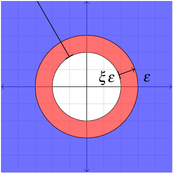
Fortunately, it’s not too hard to come up with a way to get around this. If $\mathbf{y} = 0$ is the problematic point, just leave it out! More specifically, you can cut out a small region around that singularity, do the integral over the rest of the plane, and then see if it’s well-defined in the limit as the excised region shrinks to zero. This is called cutoff regularization, and it’s the simplest of several techniques that you can use to force sensible results out of combinations of divergent integrals.

So instead of integrating over the entire plane, we’re integrating over $x > \epsilon$ or $y > \epsilon$ for some value $\epsilon$ that is the radius of the “hole” around the singularity.

$$\iint_{x > \epsilon} \uddc\mathbf{x}\frac{e^{-x^2}}{x^2}e^{-i\mathbf{k}\cdot\mathbf{x}} - \iint_{y > \epsilon} \frac{\uddc\mathbf{y}}{y^2}e^{-i\xi\mathbf{k}\cdot\mathbf{y}}$$

Now we can change variables to $\mathbf{x}$ in the second integral and keep track of what happens at the boundary of the integration region. (There’s also an outer boundary at $\infty$ to worry about, but the function is zero there so that one actually doesn’t matter. But you could use cutoff regularization on that as well.)

$$\iint_{x > \epsilon} \uddc\mathbf{x}\frac{e^{-x^2}}{x^2}e^{-i\mathbf{k}\cdot\mathbf{x}} - \iint_{x > \xi\epsilon} \frac{\uddc\mathbf{x}}{x^2}e^{-i\mathbf{k}\cdot\mathbf{x}}$$

We’ll have to correct for the difference between the two regions of integration. Suppose $\xi < 1$, then you can split the second integral into two pieces: one over $\xi\epsilon < x < \epsilon$ and one over $\epsilon < x$.

Integration regions

The first of these is the term you’d miss by taking the naive approach I described at the beginning.

$$\iint_{x > \epsilon} \uddc\mathbf{x}\frac{e^{-x^2}}{x^2}e^{-i\mathbf{k}\cdot\mathbf{x}} - \iint_{x > \epsilon} \frac{\uddc\mathbf{x}}{x^2}e^{-i\mathbf{k}\cdot\mathbf{x}} - \iint_{\xi\epsilon}^{\epsilon} \frac{\uddc\mathbf{x}}{x^2}e^{-i\mathbf{k}\cdot\mathbf{x}}$$

Finally, it’s safe to combine the first two integrals, getting the same result as before. And in the last term, we can use the series expansion of the integrand at $x\approx 0$ to do it by hand. I’ll skip the details, though, and just offer up the answer:

$$-\pi\Gamma\biggl(0, \frac{k^2}{4}\biggr) - 2\pi\ln\xi$$

This shows the dependence on $\xi$, as it should. So this expression is a nice, sensible answer.

If you were really thinking, you might have wondered why we had to impose the same cutoff, $\epsilon$, on both integrals. After all, they’re over different variables; why should their boundaries necessarily have any relation to each other? Well, that’s just the way cutoff regularization works. You could just as well use a different regularization procedure where you cut off one integral at $\epsilon$ and the other at $2\epsilon$, and you’d get a different answer. Technically, all we’ve really done is take the arbitrariness out of the singularities and move it into the regularization procedure. That really doesn’t matter, though; what’s more important is that different calculations are done using the same method of regularization, so that they’re all consistent with each other.