About a month ago, this happened: a Tesla Model S (electric car) ran over a large piece of metal which punctured its battery compartment, and the car caught on fire. It was a big deal because, according to CEO Elon Musk’s blog post (first link above), that was the first time a Tesla has caught on fire.

Since then there have been two more similar incidents in which a Tesla was involved in an accident and caught fire. Naturally, people are getting concerned: three high-profile fires in one month is a lot! But these incidents get more than their share of attention because electric cars are new technology without a proven safety record. So the question we all should be asking is, how does the fire risk in a Tesla compare to that of a regular, gas-powered car?

Most of Elon’s blog post about the first incident discusses how well the safety features of the car performed after it did catch on fire, and how this would have been a catastrophic event if the car were gas-powered like a normal car, and now we should all be driving electric cars and so on. My interest here is purely in the statistics, though. Towards the end, he points out

The nationwide driving statistics make this very clear: there are 150,000 car fires per year according to the National Fire Protection Association, and Americans drive about 3 trillion miles per year according to the Department of Transportation. That equates to 1 vehicle fire for every 20 million miles driven, compared to 1 fire in over 100 million miles for Tesla. This means you are 5 times more likely to experience a fire in a conventional gasoline car than a Tesla!

Is that true? Could you really tell, based on that one occurrence of a Tesla fire, that you’re really five times more likely to experience a fire in a gas-powered car? What about now, that there have been two more — is this enough to reach a statistically significant conclusion?

True Probability vs. Results: The Law of Large Numbers

One of the things to know about statistical significance is that it only tells you about when you can reject a hypothesis. And for that, you need a hypothesis. Statistics won’t invent the hypothesis for you — that is, it won’t tell you what your data means. You have to first come up with your own possible conclusion, some model that tells you the probabilities of various results, and then a statistical test will help you tell whether it’s reasonable or not.

The hypothesis we want to test in this case is the statement “you are 5 times more likely to experience a fire in a conventional gasoline car than a Tesla.” But to get a proper model that we can use statistical analysis on, we have to be a bit more precise about what that statement means. And in order to do that, there is one very important thing you have to understand:

The probability of something happening is not the same as the fraction of times it actually happens

This can be a tricky distinction, so bear with me. Here’s an example: Teslas have covered a hundred million miles on the road. They have experienced three fires. So you might want to conclude, based on that data, that the probability per mile of having a Tesla fire is three hundred-millionths.

But if you had done the same thing a month ago, that same reasoning would lead you to conclude that the probability per mile is one hundred-millionth! That doesn’t make any sense. The true probability per mile of experiencing a Tesla fire, whatever it is, can’t have tripled in a month! Clearly, figuring out that true probability is not as simple as just taking the fraction of times it happened.

In fact, the true probability of an event is something we don’t know, and in fact can never really know, because there’s always some variation in how many times a random event actually happens. We can only estimate the probability based on the results we see, and hope that with enough data, our estimate will be close to whatever the actual value is. It works because, as you collect more data, your estimate of the probability tends to get closer to the true probability. This statement goes by the name of the Law of Large Numbers among mathematicians.

A quick side note: you might notice that there are actually two unknown probabilities here, the true probability per mile of experiencing a fire in a gas car, and the true probability per mile of experiencing a fire in a Tesla. You can do all the right math with two unknown probabilities, but it gets complicated. To keep things from getting too crazy, I’m going to pretend that we know one of these: that the true probability for a gas car to catch on fire is five hundred millionths per mile. There’s a lot of data on gas cars, after all, and that should be a pretty precise estimate.

Step 1: Defining a Quantitative Hypothesis

With that in mind, take another look at the hypothesis.

you are 5 times more likely to experience a fire in a conventional gasoline car than a Tesla!

To rephrase, Elon is saying that the probability per mile of experiencing a fire in a Tesla is one-fifth of the probability per mile of experiencing a fire in a gasoline car. But we don’t really know that, do we? After all, true probabilities can’t be measured! What we can do is make some guesses at the true probabilities, and see how well each one corresponds to the results we’ve seen. Given this, and our assumption that we know the true probability of a gas car fire, Elon’s statement says that the probability per mile of a Tesla catching on fire is one hundred millionth. That will be our hypothesis.

Moving forward, I’m going to use \(\mathcal{P}_\text{true}\) to represent the probability per mile of a Tesla fire. We don’t know what the numerical value \(\mathcal{P}_\text{true}\) is, but our hypothesis is that \(\mathcal{P}_\text{true} = \SI{1e-8}{\per mile}\). Statisticians like to call this kind of quantity a parameter, because it’s something unknown that we have to choose when constructing our hypothesis (as opposed to the probabilities of specific results, \(P(n; \lambda)\), which we’ll be calculating later).

Step 2: Calculating Probabilities of Results

According to this hypothesis, the average number of Tesla fires per hundred million miles should be one. But of course, even if the probability per mile is actually \(\SI{1e-8}{\per mile}\), over a hundred million miles there’s some chance of having two fires. Or three. Or none. It is a random occurrence, after all. We’ll need to calculate the probabilities of having some particular number of fires every hundred million miles, starting from \(\mathcal{P}_\text{true}\).

To do this, we need to use something called a probability mass function (PMF). When you have a discrete set of possible outcomes — here, various numbers of fires per hundred million miles driven — the probability mass function tells you how likely each one is relative to the others. There are many different PMFs that apply in different situations. In our case, we have something really unlikely (a fire, \(\mathcal{P}_\text{true} = \SI{1e-8}{\per mile}\)), but we’re giving it a large number of chances (\(\mathcal{N} = \SI{1e8}{mile}\)) to happen, so the relevant PMF is that of the Poisson distribution,

Here \(n\) is some number of times the event (a car fire) could actually happen, \(P(n; \mathcal{P}_\text{true})\) is the probability it will happen that number of times, and \(\mathcal{P}_\text{true}\mathcal{N}\) is the true average number of fires in a hundred million miles — the expectation value.

This plot shows the relative probabilities for an expectation value of one:

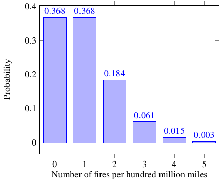
It’s important to understand just what this graph is telling you. Let’s say you decide to run an experiment, which consists of driving a car for a hundred million miles (and if it catches on fire, you swap to an identical car and keep going). And since you want to be a good scientist (you do, right?), you repeat the experiment many times to get reliable results. And suppose the underlying true probability of a car fire in this car is \(\SI{1e-8}{\per mile}\). (You wouldn’t know this value as you run the experiment, but I’m inventing this whole situation out of thin air so I can make it whatever I want.) The Poisson distribution tells you that in 36.8% of these hundred-million-mile trips, the car will not catch on fire. In another 36.8% of them, it will catch on fire once. In 18.4% of the trips, the car will catch on fire and the replacement car will catch on fire, for a total of two fires. And so on.

But it’s even more important is what this graph does not tell you. It doesn’t tell you anything about what happens if you drive a car with a different probability per mile of catching on fire.

That’s worth thinking about. It leads you to another very important thing you have to understand:

Probability tells you about the results you can get given a hypothesis, not about the hypotheses you can assume given a result

One of the most common ways people screw this up is to make an argument like this:

This hypothesis says that the probability of getting one car fire in a hundred million miles is 36.8%, so if Teslas have driven a hundred million miles and had one fire, there’s a 36.8% chance that the hypothesis is right.

But that’s just not true! The two different parts of this statement are saying very different things:

The probability of getting one car fire in a hundred million miles is 36.8%

This is the probability that the result happens, given the hypothesis. In other words, out of all the times you drive this particular type of car a hundred million miles, in 36.8% of them you will have exactly one fire.

there’s a 36.8% chance that the hypothesis is right

This, on the other hand, is talking about the probability that the hypothesis is true, given the result. In other words, out of all the times you drive the car and get one fire, it’s saying the hypothesis will be true in 36.8% of them. But that’s not the case at all! For example, think back to that same experiment I described a few paragraphs back. You drive the same kind of car a hundred million miles, many times. The hypothesis, that \(\mathcal{P}_\text{true} = \SI{1e-8}{\per mile}\), is always true in that case. So obviously, out of all the times you get one fire, the hypothesis will be true in 100% of them. That’s not 36.8%.

On the other hand, if you drive a different kind of car (with a different risk of fire) a hundred million miles, many times, you might get one fire in some of those trials, but the hypothesis will never be true. Still, that’s not 36.8%.

The point is that there’s no such thing as “the probability that the hypothesis is true.” It might always be true, it might never be true, it might be true some of the time, but in a real situation, you don’t know which of these is the case, because you don’t know the underlying parameter \(\mathcal{P}_\text{true}\). So if we’re going to evaluate whether the hypothesis is sensible, we need to do it using something other than probability.

Step 3: Likelihood-Ratio Testing

Naturally, statisticians have a tool for evaluating hypotheses. It’s called likelihood ratio testing, which is a fancy-sounding name for something that’s actually quite simple. The idea is that instead of picking a fixed value for the parameter (in our case, the true probability of a fire per mile) when you make your hypothesis, you instead try a bunch of different values. For each one, you can calculate the probability of seeing the results you actually got, given that value of the parameter, and call it the likelihood of that parameter. Likelihood is just the same number as probability, in a different context. Then comparing those different likelihoods tells you something about how likely one value of the parameter is relative to another.

Take a look at these graphs.

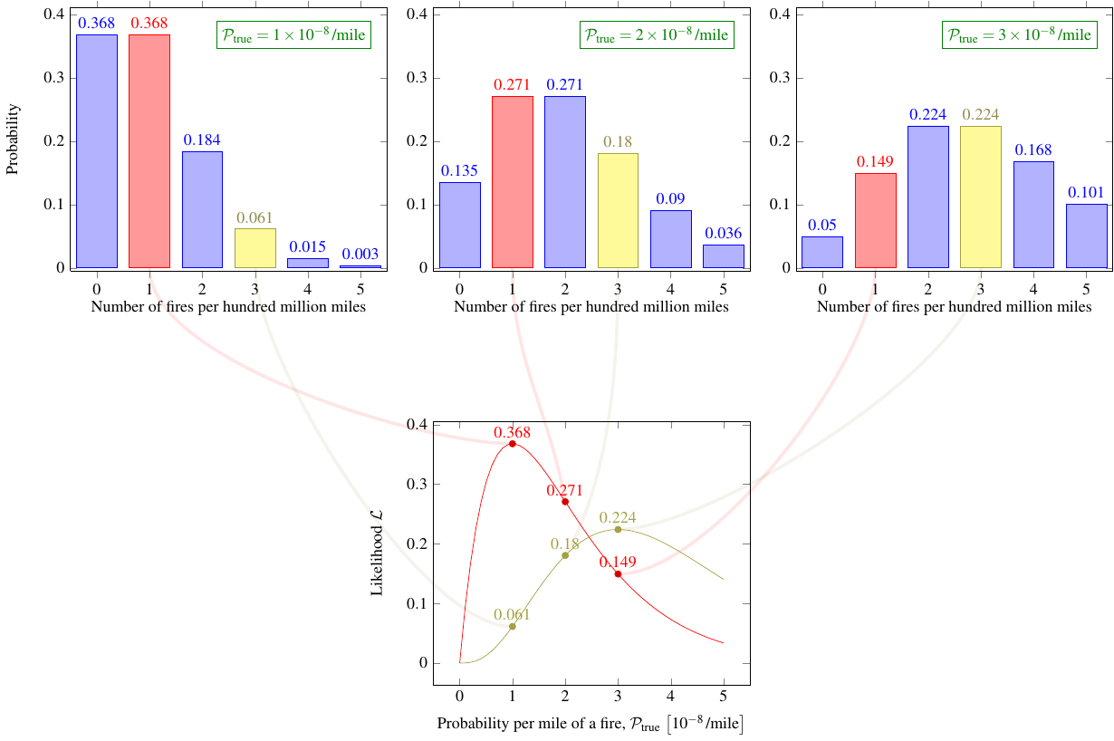
The ones on top, like the earlier graph, show the probability \(P(n; \lambda)\) of various numbers of fires, \(n\). Each graph corresponds to a different value of the parameter \(\mathcal{P}_\text{true}\). In each of the top graphs individually, all the bars add up to 1, as they should because out of all the possible outcomes, something has to happen.

The bottom graph gives you the same calculation, but this time it shows how the probability — now called likelihood — of getting a fixed number of fires changes as you adjust the parameter. In other words, each curve on the bottom graph is comparing the ability of different hypotheses to produce the same outcome. The likelihood values for a given outcome don’t have to add up to 1, because these are not mutually exclusive outcomes of the same experiment; they’re the same possible outcome in entirely different experiments.

So what can we tell from this likelihood graph? Well, for starters, hopefully it makes sense that, assuming a given result, the most likely value of the parameter (\(\mathcal{P}_\text{true}\), in this case) should be the one that has the highest likelihood — the maximum of the graph. This seemingly self-evident statement has a name, maximum likelihood estimation, and it’s actually possible to mathematically prove that, in a particular technical sense, it is the best guess you can make at the unknown value of the parameter.

The maximum likelihood method is telling us, in this case, that when there was only one Tesla fire in a hundred million miles driven, our best guess at \(\mathcal{P}_\text{true}\) was \(\SI{1e-8}{\per mile}\), based on the red curve. Now that there have been three fires in a hundred million miles driven, our best guess is revised to \(\SI{3e-8}{\per mile}\), using the yellow curve. So far, so good.

Interlude: a Toy Example

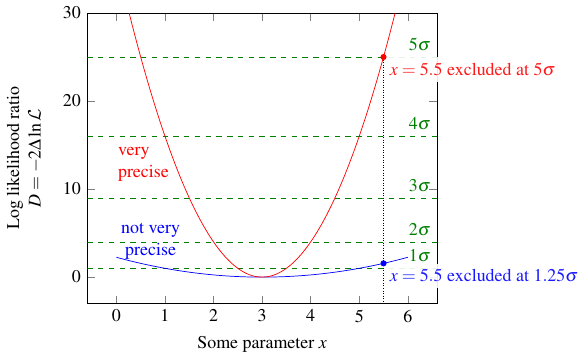
We can do more than just picking out the most likely value, though. I’ll demonstrate with an example. Have a look at these other two likelihood graphs, which I just made up out of thin air. They don’t have anything to do with the cars.

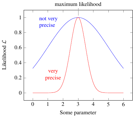
They both have the same maximum likelihood; that is, both the blue and the red curve are highest when the parameter is 3, so that’s clearly the maximum likelihood estimate — the “best guess”.

But the blue curve is very broad, so that other, widely separated values of the parameter also have fairly high likelihoods. For example, it could reasonably be 1 or 5. Thus we can’t be very confident that the true value really is close to 3.

On the other hand, the red curve is very narrow. Only values very close to the the maximum likelihood estimate have a high likelihood; values like 1 and 5 are very unlikely indeed.

Statisticians like to display this by graphing the “log likelihood ratio,” defined as the logarithm of the ratio of the likelihood to the maximum likelihood, or in math notation:

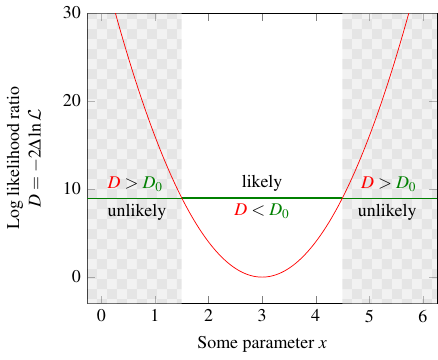
Don’t ask me why it’s called \(D\). Anyway, the plot looks like this:

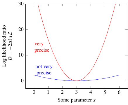
The graph kind of evokes the image of a hole that you’re dropping a ball into. If the hole is narrow, the ball is stuck pretty close to the bottom, but if the hole is wide, it has some freedom to roll around. Similarly, a narrow log likelihood ratio curve means that any reasonable estimate you can make for the value of the parameter is “stuck” near the most likely value, but a wide curve means there’s a wide range of reasonable estimates, for some definition of “reasonable.”

As you might imagine, there are various possible definitions of “reasonable,” depending on how precise you want your statistical test to be. In practice, what you actually do is pick a threshold value of \(D\). Call it \(D_0\). It splits all the possible values of the parameter, the \(x\) axis, into three regions: a central one, where \(D\) is smaller than your threshold \(D_0\), and two outer ones, where \(D\) is larger than \(D_0\).

Then you go out and run the experiment again, find some result, and calculate the corresponding value of the parameter. Assuming the maximum likelihood estimate (the bottom of the curve) is right, the value you calculated has a certain probability of falling within the center region. If \(D_0 = 1\), the probability is about 68%. If \(D_0 = 4\), it’s about 95%, because the center region is bigger. And so on.

If you pick a really high threshold, it’s really really likely that in any future experiments, the value of the parameter you calculate will be in the center region. And in turn, because those values should cluster around the true value, that means the true value should also fall in the center region! You’ve basically excluded values of the parameter outside that center — in other words, you can reject any hypothesis that has the value of the parameter outside your center region! The higher your threshold, the more confident you are in that exclusion. The probability associated with \(D_0\) is basically the fraction of times it will turn out that you were right to reject the hypothesis.

By the way, you might recognize the probabilities I mentioned above: 68% in the center for \(D_0 = 1\), 95% in the center for \(D_0 = 4\), and so on. If you have some normally distributed numbers, then 68% of the results are within \(1\sigma\) (one standard deviation) of the mean, 95% are within \(2\sigma\) of the mean, and so on. In this case, the numbers come from the chi-squared distribution, with one degree of freedom because there is one parameter, but the formula happens to work out the same, so you can make a correspondence between the threshold \(D_0\) and the number of sigmas:

If you’ve ever heard of the famous \(5\sigma\) threshold in particle physics, this is where it comes from. (At last!) A “discovery” in particle physics corresponds to choosing \(D_0 = 25\), and doing more and more experiments to narrow down that center region until it excludes whatever value of the parameter would mean “the particle does not exist.” For example, the blue curve below might represent a preliminary result of your experiment, where you exclude the value 5.5 at \(1.25\sigma\) (which is really saying nothing). The red curve might represent a final result, where you can now exclude 5.5 at \(5\sigma\) — that means the probability of the true value differing from the “best guess” (3) by 2.5 or more is less than 1 in 300 million!

At this point, hopefully you understand why it’s so hard to get a straight explanation out of a physicist as to what they mean by “discovered!”

Testing the Teslas

Now that I’ve explained (and hopefully you understand, but it’s okay if you don’t because this is complicated) how likelihood ratio testing works, and what it means to exclude a hypothesis at a certain level, let’s see how this works for the Tesla fires.

If I go back to the graph of likelihood for the Tesla fires, and compute the corresponding log likelihood ratio \(D\), I get this:

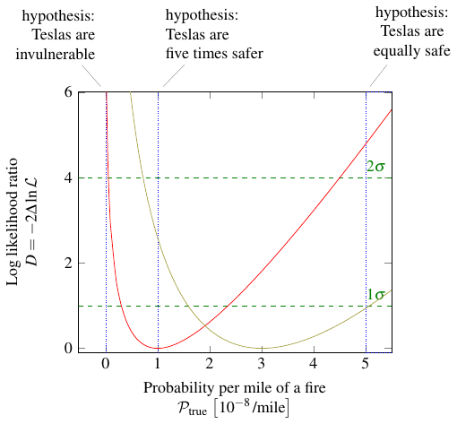
Remember, the red curve represents how the probability of having one fire per hundred million miles varies as we adjust our guess at the true probability of a fire. The yellow curve is the same except it’s for three fires per hundred million miles. We would have used the red curve a month ago, after the first fire; as of today, we should use the yellow one.

I’ve also marked three possible hypotheses — that is, three possible true values of the parameter \(\mathcal{P}_\text{true}\) — with vertical lines (or in one case a shaded area). Well, actually one of them isn’t a possible hypothesis, physically speaking. Clearly Teslas are not invulnerable; we know \(\mathcal{P}_\text{true} \neq 0\) because otherwise there would never have been any fires at all! But even if common sense didn’t tell you that, the graph would. Notice how both the red curve and the yellow curve shoot up to infinity as \(\mathcal{P}_\text{true} \to 0\). That means, no matter what threshold \(D_0\) you choose, \(\mathcal{P}_\text{true} = 0\) is always excluded (\(D > D_0\)).

Let’s now look at Elon’s original hypothesis, that Teslas are five times safer than gas cars. At that point in the graph, the red curve is zero. So Elon was perfectly justified in saying that Teslas were five times less likely to experience a fire, based on the data he had after the first fire a month ago. These days, however, it wouldn’t be quite so easy to make that claim. The yellow curve, the one based on the three fires we’ve seen so far, has a value of \(D = 2.59\). That means the hypothesis is excluded at the \(1.6\sigma\) level (because \(1.6 = \sqrt{2.59}\)), or that there is an 11% probability of seeing something at least as extreme as the observed result (three fires) given that hypothesis. That’s not a small enough percentage to rule out the hypothesis by any common standard, so it’s still potentially viable — just not as likely as it used to be.

If you ask me, though, the really important question is this: do Teslas have a lower fire risk than gas cars, period? To that end, I included the third hypothesis, that Teslas are just as safe than normal cars. That’s the dotted line on the right. Based on the data from a month ago, after the first car fire, that hypothesis is excluded at the \(2\sigma\) level — actually, it’s \(2.18\sigma\), but it’s common to round down. That corresponds to a 3% probability of seeing only one fire (or some even more extreme result), if the hypothesis is correct; in a sense, this also means that if you decided to go ahead and declare the Tesla safer than a gas car, you’d have a 3% chance of being wrong. For a lot of people outside particle physics, that’s good enough; 5% (or \(D_0 = 4\), remember) is a common cutoff. But 5% is still not that small. It means you’re wrong one out of every 20 times on average.

Fast forward to today, and we now have to use the yellow curve. That intersects the hypothesis line quite a bit lower; in fact, it’s less than one sigma! So based on current data, if you decide to reject the hypothesis that Teslas are as safe as gas cars, you have a one in three chance of being wrong. Either way, I don’t think anyone would consider it safe to reject that hypothesis based on that result. For now, we have to live with the possibility that Teslas may not have any lower of a fire risk than regular gas-powered cars. Sorry, Elon.