Time to kick off a new year of blog posts! For my first post of 2015, I’m continuing a series I’ve had on hold since nearly the same time last year, about the research I work on for my job. This is based on a paper my group published in Physical Review Letters and an answer I posted at Physics Stack Exchange.

In the first post of the series, I wrote about how particle physicists characterize collisions between protons. A quark or gluon from one proton (the “probe”), carrying a fraction \(x_p\) of that proton’s momentum, smacks into a quark or gluon from the other proton (the “target”), carrying a fraction \(x_t\) of that proton’s momentum, and they bounce off each other with transverse momentum \(Q\). The target proton acts as if it has different compositions depending on the values of \(x_t\) and \(Q\): in collisions with smaller values of \(x_t\), the target appears to contain more partons.

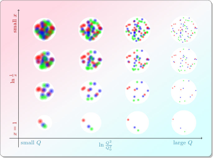
At the end of the last post, I pointed out that something funny happens at the top left of this diagram. Maybe you can already see it: in these collisions with small \(x_t\) and small \(Q\), the proton acts like a collection of many partons, each of which is relatively large. Smaller \(x_t\) means more partons, and smaller \(Q\) means larger partons. What happens when there are so many, and so large, that they can’t fit?

Admittedly, that may not seem like a problem at first. In the model I’ve been using so far, a proton is a collection of particles. And it seems totally reasonable that when you’re looking at a proton from one side, some of the particles will look like they’re in front of other particles. But this is one of those situations where the particle model falls short. Remember, protons are really made of quantum fields. Analyzing the proton’s behavior using quantum field theory is not an easy task, but it’s been done, and it turns out an analogous, but very serious, problem shows up in the field model: if you extrapolate the behavior of these quantum fields to smaller and smaller values of \(x_t\), you reach a point where the results don’t make physical sense. Essentially it corresponds to certain probabilities becoming greater than 1. So clearly, something unexpected and interesting has to happen at small \(x_t\) to keep the fields under control.

Parton branching and the BFKL equation

To explain how we know this, I have to go all the way back to 1977. Quantum chromodynamics (QCD), the model we use to describe the behavior of quarks and gluons, was only about 10 years old, and physicists at the time were playing around with it, poking and prodding, trying to figure out just how well it explained the known behavior of protons in collisions.

Most of this tinkering with QCD centered around the parton distributions \(f_i(x, Q^2)\), which I mentioned in my last post. Parton distributions themselves actually predate QCD. They first emerged out of something called the “parton model,” invented in 1969, which is exactly what it sounds like: a mathematical version of the statement “protons are made of partons.” So by the time QCD arrived on the scene, the parton distributions had already been measured, and the task that fell to the physicists of the 1970s was to try to reproduce the measurements of \(f_i(x, Q^2)\) using QCD.

When you’re testing a model of particle behavior, like QCD, you do it by calculating something called a scattering cross section, which is like the effective cross-sectional area of the target particle. If the target were a sphere of radius \(r\), for example, its cross section would be \(\pi r^2\). But unlike a plain old solid sphere, the scattering cross section for a subatomic particle depends on things like how much energy is involved in the collision (which you may remember as \(\sqrt{s}\) from the last post) and what kinds of particles are colliding. The information about what kinds of particles are colliding is represented mathematically by the parton distributions \(f_i(x, Q^2)\). So naturally, in order to make a prediction using the theory, you need to know the parton distributions.

The thing is, we actually can’t do that! Believe me, people are trying, but there’s a fairly fundamental problem: parton distributions are nonperturbative, meaning they are inextricably linked to the behavior of the strong interaction when it is too strong for standard methods to handle. They already knew this in the 1970s. However, that didn’t stop people from trying to calculate something about the PDFs which could be linked to experimental results.

It turns out that even though the exact forms of the parton distributions can’t be calculated from quantum field theory, you can calculate their behavior at small values of \(x\), the green part on the left of the preceding diagram. In 1977, four Russian physicists — Ian Balitsky, Victor Fadin, Eduard Kuraev and Lev Lipatov — derived from QCD an equation for the rate of change of parton distributions with respect to \(x\), in collisions with energy \(\sqrt{s}\) much larger than either the masses of the particles involved or the amount of energy transferred between them (\(Q\), roughly). In modern notation, the equation (which I will explain later) is written

\(N\) is something called the color dipole cross section, which is related to \(f\) from before via an equation roughly like this:

That’s why \(f\) is often called an integrated parton distribution and \(N\) an unintegrated parton distribution. I won’t go into the details of the difference between \(N\) and \(f\), since both of them show the behavior I’m going to talk about in the rest of this post.

Anyway, the behavior that Balitsky, Fadin, Kuraev, and Lipatov analyzed comes from processes like these:

At each vertex, one parton with a certain fraction \(x\) of the proton’s momentum splits into other partons with smaller values of \(x\). You can see this reflected in the equation: the term \(-N(x, Q^2, \vec{r}_{01})\) represents the disappearance of the original parton, and \(N(x, Q^2, \vec{r}_{02}) + N(x, Q^2, \vec{r}_{12})\) represents the creation of two new partons with smaller momentum fractions \(x\). When this happens repeatedly, it leads to a cascade of lower-and-lower momentum particles as the branching process goes on. This explains why the number of partons, and thus the parton distribution functions, increase as you go to smaller and smaller values of \(x\).

This BFKL model has been tested in experiment after experiment for many years, and it works quite well. For example, in the plot below, from this paper by Anatoly Kotikov, you can see that the predictions from the BFKL equation (solid lines) generally match the experimental data (dots with error bars) quite closely.

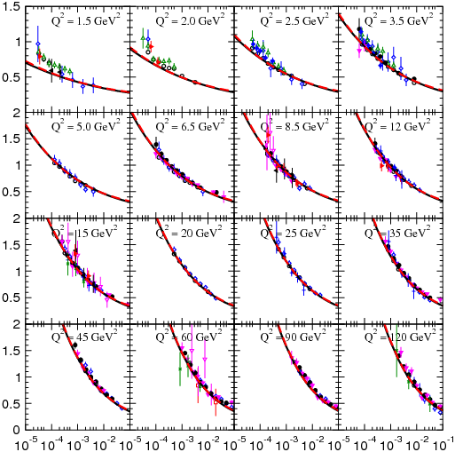
The plot shows the structure function \(F_2\), which is a quantity related to the integrated parton distribution.

Parton recombination

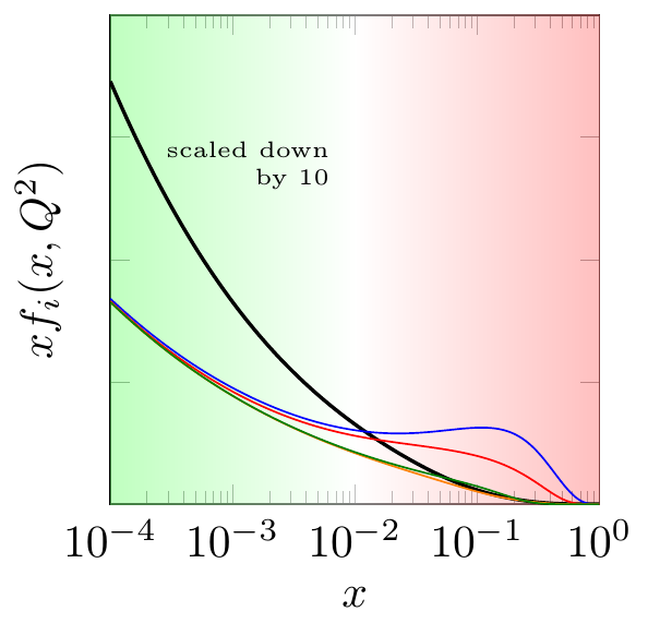
However, there is one big problem with the BFKL prediction: it never stops growing! After all, if the partons keep splitting over and over again, you keep getting more and more of them as you go to lower momentum fractions \(x\). Mathematically, this corresponds to exponential growth in the parton distributions:

which is roughly the solution to the BFKL equation.

If the parton distributions get too large, when you try to calculate the scattering cross section, the result “breaks unitarity,” which effectively means the probability of two partons interacting becomes greater than 1. Obviously, that doesn’t make sense! So this exponential growth that we see as we look at collisions with smaller and smaller \(x_t\) can’t continue unchecked. Some new kind of physics has to kick in and slow it down. That new kind of physics is called saturation.

The physical motivation for saturation was proposed by two physicists, Balitsky (the same one from BFKL) and Yuri Kovchegov, in a series of papers starting in 1995. Their idea is that, when there are many partons, they actually interact with each other — in addition to the branching described above, you also have the reverse process, recombination, where two partons with smaller momentum fractions combine to create one parton with a larger momentum fraction.

At large values of \(x\), when the number of partons is small, it makes sense that not many of them will merge, so this recombination doesn’t make much of a difference in the proton’s structure. But as you move to smaller and smaller \(x\) and the number of partons grows, more and more of them recombine, making the parton distribution deviate more and more from the exponential growth predicted by the BFKL equation. Mathematically, this recombination adds a negative term, proportional to the square of the parton distribution, to the equation.

When the parton density is low, \(N\) is small and this nonlinear term is pretty small. But at high parton densities, the nonlinear term has a value close to 1, which cancels out the other terms in the equation. That makes the rate of change \(\pd{N}{\ln\frac{1}{x}}\) approach zero as you go to smaller and smaller values of \(x\), which keeps \(N\) from blowing up and ruining physics.

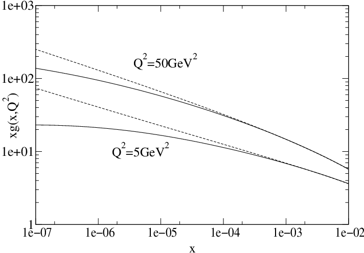
By way of example, the following plot, from this paper (my PhD advisor is an author), shows how the integrated gluon distribution grows more slowly when you include the nonlinear term (solid lines) than when you don’t (dashed lines):

So where does that leave us? Well, we have a great model that works when the parton density is low, but we don’t know if it works when the density is high. That’s right: saturation has never really been experimentally confirmed, although it’s getting very close. In the third and final post in this series (not counting any unplanned sequels), I’ll explain how physicists are now trying to do just that, and how my group’s research fits into the effort.